
The cost of a chip starts with a simple division: the cost of a processed wafer divided by the number of good dies on it. That number depends on two things that physical design controls more than any other step: the die area, which sets how many dies fit on the wafer, and the area exposed to defects, which sets how many of them work. This article counts dies on a 300 mm wafer, compares three yield models, and works out the cost of a good die for four die sizes, with every assumption stated.
7 min read | Intermediate
What You'll Learn
- Count gross dies on a wafer, by formula and by placement
- Compare the Poisson, Murphy and negative binomial yield models
- Compute the cost of a good die and the total cost of a part
- Explain why die area matters more than linearly
The Cost Equation
The manufacturing cost of one part is the sum of three terms:
cost per part = process cost + package cost + test cost
process cost  = wafer cost / (dies per wafer x die yield x packaging yield)
The wafer cost covers everything from wafer start to wafer out. The dies per wafer is the number of complete dies that fit, called the gross dies. The die yield is the share of those that work. The packaging yield, typically 95 to 99 %, covers losses in assembly and final test.
The rest of this article uses one set of assumptions, chosen for illustration and stated here so the numbers can be recomputed: a 300 mm wafer, a 3 mm edge exclusion, a 0.1 mm scribe lane, a defect density D0 of 0.2 defects per cm2 and a wafer cost of $5,000. Real values are set by the foundry and the process and are rarely published.
How Many Dies Fit
A first estimate divides the wafer area by the die area and subtracts the partial dies along the edge:
gross dies = pi x (d/2)^2 / A - pi x d / sqrt(2 x A)
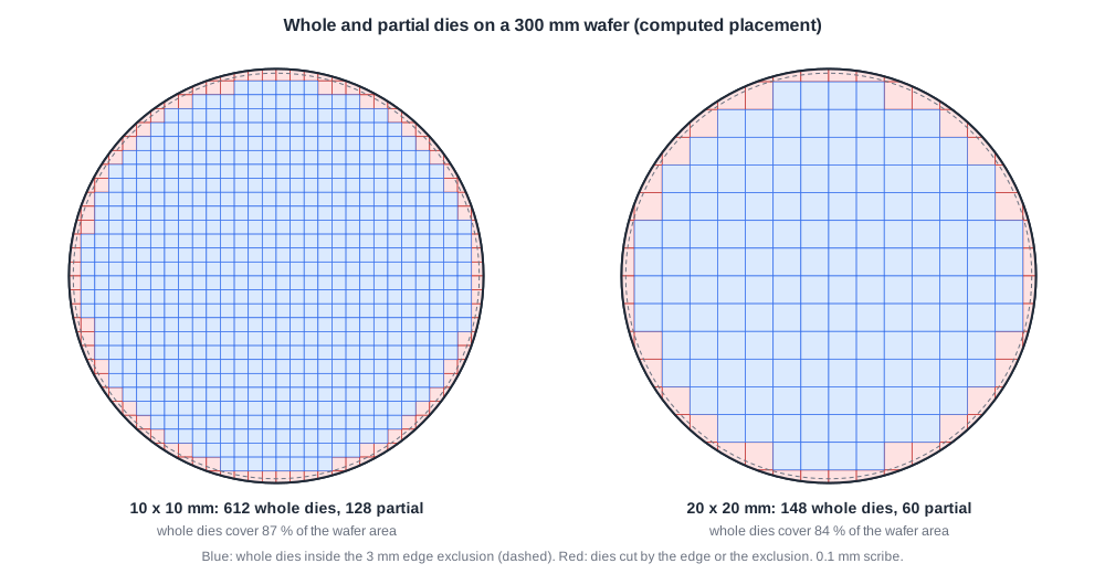
where d is the wafer diameter and A the die area including its share of the scribe lane. Counting the dies that actually fit, by placing a grid of dies on the usable circle and keeping only complete ones, gives:
| Die | Area | Formula | Placed on the wafer |
|---|---|---|---|
| 1 x 1 mm | 1 mm2 | 57,812 | 55,631 |
| 5 x 5 mm | 25 mm2 | 2,587 | 2,502 |
| 10 x 10 mm | 100 mm2 | 627 | 612 |
| 20 x 20 mm | 400 mm2 | 142 | 148 |
The formula ignores the edge exclusion, so it is a little high for small dies, and it is only an estimate of the edge loss, so for large dies a good placement can beat it. Either way, the edge costs more as the die grows: a 20 mm die loses a large share of the wafer rim.
Quick Check
Q: The die area grows four times from 5 x 5 mm to 10 x 10 mm. Why does the number of placed dies fall by slightly more than four, from 2,502 to 612?
Show Answer
Area alone would give a factor of four. The larger die also wastes more of the round edge, where partial dies cannot be used. 2,502 / 612 is about 4.1; the extra loss is the edge.
Three Yield Models
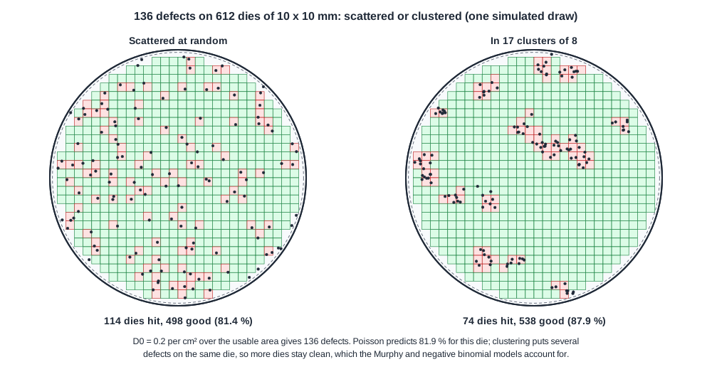
Design for Manufacturing and Yield introduced the Poisson model, which assumes defects are scattered independently over the wafer. Real defects cluster: some wafers, some regions and some lots have many, others few. Clustering leaves more dies untouched for the same average density, so the Poisson model is pessimistic for large dies. Two common alternatives account for it:
Poisson:            Y = exp(-A x D0)
Murphy:             Y = ((1 - exp(-A x D0)) / (A x D0))^2
negative binomial:  Y = (1 + A x D0 / alpha)^(-alpha)
The clustering factor alpha in the negative binomial model is fitted to a fab's data: a small alpha means strong clustering, and as alpha grows the model approaches Poisson. The chart uses alpha = 2.
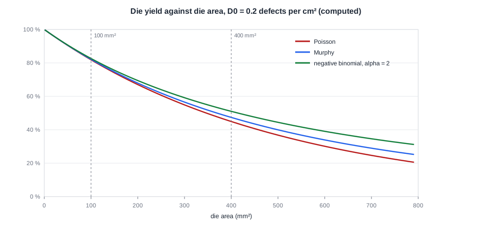
For small dies the three models agree: A x D0 is small and almost every die is defect-free. For a 400 mm2 die they give 44.9 %, 47.4 % and 51.0 %. Which model to trust is a question for the foundry's data, but the trend is the same in all three: yield falls faster than area grows.
The Cost of a Good Die
Multiplying placed dies by the negative binomial yield and dividing the wafer cost by the result:
| Die | Placed dies | Yield | Good dies | Wafer cost per good die |
|---|---|---|---|---|
| 1 x 1 mm | 55,631 | 99.8 % | 55,520 | $0.09 |
| 5 x 5 mm | 2,502 | 95.2 % | 2,382 | $2.10 |
| 10 x 10 mm | 612 | 82.6 % | 506 | $9.88 |
| 20 x 20 mm | 148 | 51.0 % | 75 | $66.67 |
From 5 mm to 10 mm the area grows four times and the cost per good die almost five times; from 10 mm to 20 mm the area grows four times and the cost almost seven times. This is the economic reason behind many physical design choices: a utilization a few percent higher, a smaller core margin or a tighter floorplan saves more than its share of area, and a design that can be split into smaller dies, as chiplets do, can be cheaper even with the packaging overhead.
Package and test costs come on top. For a small die they can exceed the silicon cost; for a large one the silicon dominates. Test cost grows with test time, which is one reason why test programs are optimized as carefully as the layout.
Quick Check
Q: Two designs have the same function. One is a single 20 x 20 mm die; the other is four 10 x 10 mm dies in one package. Using the table, compare their wafer cost per working set.
Show Answer
The large die costs $66.67 per good die. Four tested 10 mm dies cost 4 x $9.88 = $39.52. The split version is cheaper in silicon, as long as the multi-die package and the extra testing cost less than the $27 difference, and the dies are known good before assembly.
Beyond Random Defects
The models above cover random defects only. In practice yield has more parts:
- Systematic yield. Patterns that print or polish badly fail on every wafer; they show up as a fixed loss that DFM and lithography checks attack.
- Parametric yield. Dies that work but miss their speed or power target at test. Timing margin across corners, as checked in sign-off, protects it.
- Learning. The defect density of a new process falls over its first months and years of production, so the same die becomes cheaper over time.
- Repair. Memories with spare rows and columns, and chips with spare cores, turn some defective dies into good ones.
Running It in ChipVerify Lab
Run Place and Route on the multiplier and read the die size: 175.465 um square, or 0.031 mm2. At 0.2 defects per cm2 its Poisson yield is 99.994 %. For a die this small, the scribe lane is the bigger loss: with a 0.1 mm lane, each die occupies a 0.275 mm square on the wafer, and only 41 % of that is the die itself. Real dies are many times larger, so their scribe share is small and their defect share large.
Common Mistakes
Mistake #1: Treating cost as proportional to area
Fewer dies fit and fewer of them work as area grows, so cost per good die rises faster than area.
Mistake #2: Using one yield model without data
The models agree for small dies and differ for large ones. For large dies, use the foundry's model and parameters.
Mistake #3: Forgetting package and test costs
For small dies they can be the larger share of the part cost.
Practice Exercise
Challenge: A 7 x 7 mm Die
With the assumptions of this article, 1,273 dies of 7 x 7 mm fit on the wafer. What is the Poisson yield at 0.2 defects per cm2, how many good dies does a wafer give, and what is the wafer cost per good die at $5,000 per wafer? With a 98 % packaging yield, what is the process cost per packaged part?
Hint
0.2 defects per cm2 is 0.002 per mm2; the die area is 49 mm2.
Solution
A x D0 = 49 x 0.002 = 0.098, so Y = exp(-0.098) = 90.7 %. Good dies: 1,273 x 0.907 = 1,155. Wafer cost per good die: $5,000 / 1,155 = $4.33. Process cost per packaged part: $4.33 / 0.98 = $4.42.
Open the ready-made example in the lab, synthesize it and run Place and Route.
Summary
- Process cost per part is the wafer cost divided by gross dies, die yield and packaging yield; package and test costs add to it.
- Gross dies fall slightly faster than area grows, because large dies waste more of the wafer edge.
- Poisson, Murphy and negative binomial models agree for small dies; clustering makes the last two more optimistic for large ones.
- With the stated assumptions, quadrupling the area from 10 to 20 mm square raises the cost per good die almost seven times.
- Systematic and parametric yield, learning and repair add to the random-defect picture.
