
Placement decides where every standard cell goes, and with it the length of almost every wire. Global placement is the first step: it spreads the cells over the core so that connected cells are close together and no region is overfull. It does not care yet about exact sites or overlaps. This article explains the two goals global placement balances, wire length and density, and reads the progress of OpenROAD's global placer, RePlAce, on the multiplier.
8 min read | Intermediate
What You'll Learn
- Explain the two competing goals of global placement
- Define half-perimeter wire length (HPWL) and overflow
- Read the global placement log of OpenROAD
- Choose a target density and predict its effect
Two Goals
If wire length were the only goal, the best placement would put every cell on the same spot: all wires would have zero length. If spreading were the only goal, the cells would be scattered evenly with no regard for their connections. Global placement minimizes wire length subject to a density limit: in every small region of the core, the cells may fill at most a target fraction of the area.
OpenROAD's global placer treats the cells like electric charges. Overfull regions create a "field" that pushes cells out, while the nets pull connected cells together. It starts with all cells near the centre and solves step by step, gradually increasing the weight of the density force, until the cells are spread enough.
Measuring Wire Length: HPWL
Routing is not done yet, so the placer estimates the wire length of each net from the pin positions: the half-perimeter wire length is half the perimeter of the smallest rectangle around all pins of the net, that is its width plus its height. For a net with two pins it is exactly the Manhattan distance; for nets with more pins it is a lower bound on the routed length. The total HPWL is the sum over all nets.
Measuring Spreading: Overflow
The core is divided into bins, for the multiplier 32 x 32 bins of 4.84 x 4.76 um. In every bin, the placer compares the cell area with the target density times the bin area. Overflow is the share of the total cell area that sits above the target in overfull bins. 1.0 means all cells are piled up; 0 means every bin is within its limit. OpenROAD stops when overflow falls below 0.10, and the detailed placer resolves the rest.
Quick Check
Q: A net connects pins at (10, 10), (30, 15) and (20, 40) um. What is its HPWL?
Show Answer
The bounding box spans x from 10 to 30 and y from 10 to 40: HPWL = 20 + 30 = 50 um. A routed tree for these three pins needs at least that much wire.
Reading the Log
The multiplier's run starts by summing up what it has to place:
[INFO GPL-0006] Number of instances:              1586
[INFO GPL-0007] Movable instances:                1267
[INFO GPL-0008] Fixed instances:                   319
[INFO GPL-0035] Pin density area adjust:       629.354 um^2
[INFO GPL-0019] Utilization:                    44.359 %
[INFO GPL-0023] Placement target density:       0.5000
The 319 fixed instances are the tap cells. The pin density adjustment adds area to cells with many pins, so that the placer leaves room for their wires. Then the main loop prints a line every 10 iterations:
Iteration | Overflow |     HPWL (um) |  HPWL(%) |   Penalty
        0 |   0.9829 |  3.556844e+03 |   +0.00% |  1.18e-15
      200 |   0.9211 |  7.338425e+03 |  +13.33% |  2.04e-11
      300 |   0.5576 |  1.777516e+04 |   +3.83% |  2.69e-09
      450 |   0.0986 |  2.026251e+04 |          |  1.46e-06
[INFO GPL-1001] Global placement finished at iteration 450
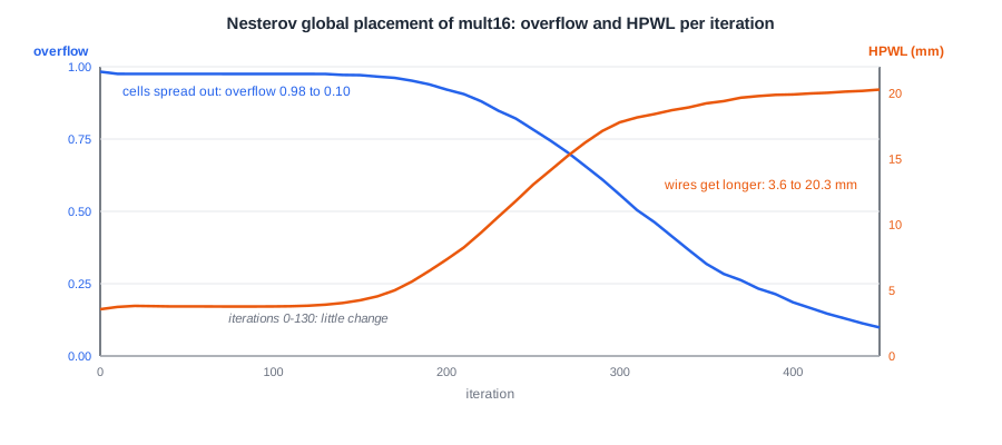
The plot shows the trade-off at work. For the first 130 iterations the penalty for density is tiny and nothing much happens: the cells stay in a tight cluster with 3.6 mm of HPWL and almost everything overflowing. As the penalty grows, the cells spread and the overflow falls, and the wire length rises with it. At the end the overflow is below 0.10 and the HPWL is 20.3 mm, almost six times the starting value. Spreading costs wire length; the placer's job is to pay as little of it as possible.
Target Density
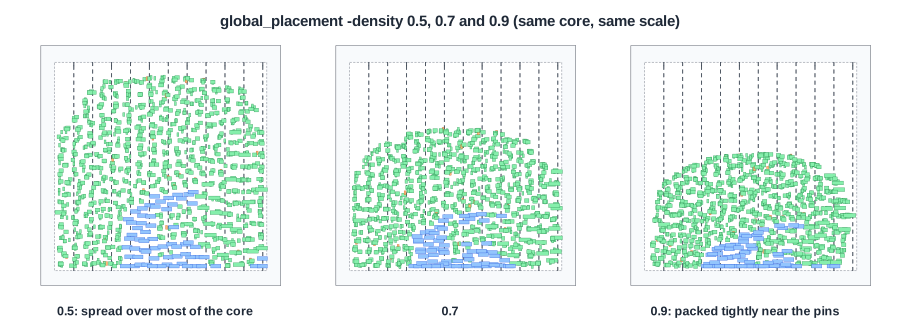
The target density is the main knob. The lab's flow derives it from the floorplan: the real core utilization plus 0.10, kept between 0.20 and 0.95, and prints it before global placement (Placement density: 0.53 (core utilization 42.6%) for the multiplier at 40 %). The same core, three targets:
| Target density | HPWL after global placement | Routed wire | Worst slack at 10 ns |
|---|---|---|---|
| 0.5 | 20.3 mm | 28.3 mm | +0.58 ns |
| 0.7 | 16.7 mm | 25.8 mm | +0.74 ns |
| 0.9 | 14.9 mm | 25.8 mm | +0.49 ns |
With a target of 0.5 the cells cover most of the core; at 0.9 they pack into a smaller region near the pins, which in this run all sit on the bottom edge. A higher target gives shorter wires, but the cells are packed more tightly than the detailed placer and the router like. From 0.7 to 0.9 the HPWL drops another 11 %, yet the routed wire length is the same and the slack is worse: the detailed placer had to move cells further (the next article has the numbers), and the router found less room.
The log helps choose the target. After placement, OpenROAD suggests values:
[INFO GPL-1004] Minimum Feasible Density        0.4500 (cell_area / free_area)
[INFO GPL-1008]     - For 80% usage of free space: 0.5545
The minimum feasible density is the utilization: a lower target cannot be met. Targets slightly above it spread the cells over the whole core; targets well above it cluster them.
Quick Check
Q: Why does a lower target density give longer wires even though the core is the same size?
Show Answer
A lower target forces the cells to spread over more of the core, so connected cells end up further apart. With a higher target they may cluster tightly, leaving the rest of the core empty.
Running It in ChipVerify Lab
Run Place and Route on the multiplier and find the GPL section of the log: the instance counts, the target density and the iteration table. Run it again at a different utilization in the panel; the core changes size and the lab's target density follows the new core utilization, so the iteration count and final HPWL change with it.
Common Mistakes
Mistake #1: Taking HPWL as the routed length
HPWL is a lower bound for nets with more than two pins, and the router adds detours. In the multiplier, 20.3 mm of HPWL became 28.3 mm of routed wire.
Mistake #2: Setting the target density as high as possible
A very high target gives the best HPWL on paper, but leaves no room for legalization, buffers and routing. Judge the target by the final routed result, not by the global placement number.
Practice Exercise
Challenge: Cells per Bin
The multiplier's bins are 4.84 x 4.76 um and its cells average 8.1 um2. At a target density of 0.5, how many average cells may one bin hold? And at 0.9?
Hint
Allowed cell area per bin = target density x bin area.
Solution
The bin area is 23.0 um2. At 0.5: 11.5 um2, about 1.4 average cells. At 0.9: 20.7 um2, about 2.6 cells. The log reports a related number, the "ideal bin area": 16.3 um2 at 0.5 and 9.0 um2 at 0.9, the bin size in which exactly one average cell fills the target.
Open the ready-made example in the lab, synthesize it and run Place and Route.
Summary
- Global placement minimizes wire length while keeping every region below a target density.
- HPWL estimates wire length from pin bounding boxes; overflow measures how much cell area sits in overfull bins.
- OpenROAD stops at an overflow of 0.10; in the multiplier that took 450 iterations and gave 20.3 mm of HPWL.
- A higher target density shortens the HPWL but makes legalization and routing harder.
