
Every setup violation in a timing report is the result of one small equation. If you can write that equation yourself, you can predict what a change to the clock or the logic does to the slack before you run the tool. This chapter takes setup and hold apart, step by step, and then shows how to fix violations.
The setup equation compares two times: when the data arrives at a flip-flop and when it must be there. This article builds the equation from the beginning, includes the clock arrival times of both flip-flops, and tests it on a real path.
8 min read | Intermediate
What You'll Learn
- Name every term of the setup equation and say where each number comes from
- Write the data arrival time and the data required time of a register-to-register path
- Explain how clock arrival times and clock skew change the setup slack
- Calculate setup slack by hand and check it against a timing report
The Question Setup Asks
A flip-flop copies the value at its D pin on the clock edge. For this to work, the new value must already be at D, and stable, a short time before the edge. That short time is the setup time of the flip-flop, and it is a number in the cell library.
The setup check asks one question about each path: does the data reach the D pin early enough? To answer it, STA calculates two times on the same time axis and compares them. The data arrival time is when the data actually reaches the pin. The data required time is the latest moment at which it is allowed to arrive.
Step 1: The Data Arrival Time
The data starts its journey when the clock edge reaches the launch flip-flop. The clock does not reach every flip-flop at time zero. It travels through wires and buffers, so each flip-flop gets it a little later. The time at which the clock edge reaches a flip-flop is called the clock arrival time, or clock latency. For the launch flip-flop we call it Tlaunch.
From that moment the data needs time to travel. First the flip-flop takes some time to change its output after the clock edge, called the clock-to-Q delay, Tclk-to-Q. Then the data goes through the logic between the two flip-flops, with the delay Tdp (delay of the data path, including the wires). So:
Data arrival time = Tlaunch + Tclk-to-Q + Tdp
Step 2: The Data Required Time
The data is captured by the second flip-flop, which has its own clock arrival time Tcapture. For the setup check the data has to be captured by the next clock edge, one clock period after the launch edge. So the capture edge reaches the capture flip-flop at Tcapture + Tperiod. The data must be stable one setup time before that, so:
Data required time = Tcapture + Tperiod - Tsetup
Step 3: Compare the Two
The setup check passes when the data arrives no later than it is required. The difference is the setup slack:
Setup check:  Tlaunch + Tclk-to-Q + Tdp  <=  Tcapture + Tperiod - Tsetup

Setup slack = (Tcapture + Tperiod - Tsetup) - (Tlaunch + Tclk-to-Q + Tdp)
Slack of zero or more means the check is met. Negative slack means the data arrives too late and the setup check is violated.
A Real Example With Skew
The difference Tcapture - Tlaunch is called clock skew. It is the amount by which the capture flip-flop gets its clock later than the launch flip-flop. If both flip-flops have an ideal clock, the skew is zero. Now give the capture flip-flop of the demo circuit a clock that is 0.3 ns late, with the constraint:
set_clock_latency 0.3 [get_pins _6_/CLK]
The name _6_ is the capturing flip-flop in our run. The clock period is 2.0 ns, the clock-to-Q delay is 0.2874 ns, the logic delay is 0.1450 ns and the setup time is 0.1174 ns. The diagram below shows the two clocks: the launch clock edge at 0.0 ns, and the capture clock, which is late by 0.3 ns. Its first edge is at 0.3 ns and the edge that counts for setup is at 2.3 ns.
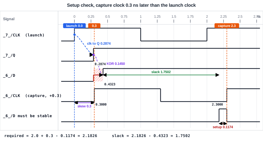
Put the numbers in the equation:
| Term | Value (ns) |
|---|---|
| Data arrival time = 0 + 0.2874 + 0.1450 | 0.4323 |
| Data required time = 0.3 + 2.0 - 0.1174 | 2.1826 |
| Setup slack = 2.1826 - 0.4323 | 1.7502 |
The timing report shows the same values. The capture clock row has a network delay of 0.3000, and the required time is 2.1826:
             0.0000    2.0000    2.0000   clock clk (rise edge)
                       0.3000    2.3000   clock network delay (ideal)
                       0.0000    2.3000   clock reconvergence pessimism
                                 2.3000 ^ _6_/CLK (sky130_fd_sc_hd__dfxtp_1)
                      -0.1174    2.1826   library setup time
                                 2.1826   data required time
                                -0.4323   data arrival time
                                 1.7502   slack (MET)
Without the skew the slack was 1.4502 ns. The late capture clock gave the data 0.3 ns more time, and the slack went up by exactly 0.3 ns. A late capture clock helps setup, and a late launch clock hurts it. That is what Tcapture - Tlaunch means in the equation. The row clock reconvergence pessimism is zero here. It is a correction for clock paths that share part of their route, explained in the chapter about variation.
Adding Margin: Clock Uncertainty
Real designs keep some extra margin because the clock edge is not perfectly steady. In the constraints this margin is called clock uncertainty, written Tuncertainty. For setup it is subtracted from the required time:
Data required time = Tcapture + Tperiod - Tsetup - Tuncertainty
The capture edge is treated as if it came earlier, so the data has less time. Clock uncertainty is covered in detail in the chapter about clocks.
What Limits the Clock Speed
Look at the equation once more. Only the clock period belongs to the clock. Everything else is a delay. So the setup check limits how short the period can be. Solve the equation for the period, with no skew and no uncertainty:
Tperiod >= Tclk-to-Q + Tdp + Tsetup
For the path above, this is 0.2874 + 0.1450 + 0.1174 = 0.5498 ns. A faster clock reduces Tperiod and makes setup slack smaller. A slower clock gives more slack.
Common Mistakes
Mistake #1: Forgetting the clock period in the required time
The data launched at one clock edge is captured at the next edge, so the required time contains a full period. Without it, nothing would ever meet the check.
Mistake #2: Mixing up the sign of the skew
Skew is the capture clock arrival minus the launch clock arrival. If the capture clock is later, setup slack goes up. If the launch clock is later, setup slack goes down. When in doubt, draw the two clocks as in the diagram above.
Quick Check: A path has a clock-to-Q delay of 0.30 ns, a logic delay of 0.90 ns and a setup time of 0.10 ns. The period is 1.5 ns and the skew is zero. What is the setup slack?
Arrival time = 0.30 + 0.90 = 1.20 ns. Required time = 1.5 - 0.10 = 1.40 ns. Slack = 1.40 - 1.20 = 0.20 ns, so the check is met.
Practice Exercise
Challenge: Predict the Slack With a Late Launch Clock
Start with the sta_demo design at a 2.0 ns period. The setup slack of the register-to-register path is 1.4502 ns. Add a delay of 0.3 ns to the clock of the launching flip-flop (_7_ in our run) instead of the capturing one:
set_clock_latency 0.3 [get_pins _7_/CLK]
Predict the new data arrival time and the new setup slack, then run STA to check your prediction.
Open the ready-made example in the lab, run synthesis, and then run STA. Editing constraints.sdc and re-running only STA, and choosing another library or corner, are PRO features.
Hint
The launch clock arrival time Tlaunch is now 0.3 ns, and nothing else in the equation changes.
Solution
The data arrival time is 0.3 + 0.2874 + 0.1450 = 0.7323 ns. The required time stays at 2.0 - 0.1174 = 1.8826 ns. The slack is 1.8826 - 0.7323 = 1.1502 ns, which is 0.3 ns less than before. A late launch clock gives the data less time.
Summary
- The setup check compares the data arrival time with the data required time.
- Data arrival time = launch clock arrival + clock-to-Q delay + logic delay.
- Data required time = capture clock arrival + clock period - setup time (minus clock uncertainty).
- Setup slack = required time - arrival time. Zero or more means met.
- Skew is the capture clock arrival minus the launch clock arrival. A later capture clock adds to the setup slack, a later launch clock takes from it.
- The setup check limits how short the clock period can be: the period must cover clock-to-Q, logic and setup time.
