
A flat OCV derate is easy to understand and easy to apply, but it is a blunt tool. It adds the same percentage to a path of one cell and to a path of thirty cells. In practice, the random differences between cells partly cancel on a long path: if one cell is slow, another is probably fast. Advanced OCV, AOCV, uses derates that become smaller as the path gets longer. This article explains the idea, shows how a derate table is read, and works through an example. The numbers in the tables are made up to show the shape, not taken from a real technology.
8 min read | Intermediate
What You'll Learn
- Explain why a flat derate is pessimistic for long paths
- Describe depth-based and distance-based derating
- Read an AOCV table and find the derate of a path
- Calculate how much margin AOCV gives back compared with a flat derate
The Problem With a Flat Derate
Suppose the random variation of each cell is up to 12 percent. A path with a single cell can be unlucky and be 12 percent slow, so a late derate of 12 percent is right for it. A path of sixteen cells is different. For all sixteen cells to be 12 percent slow at the same time is very unlikely. In real chips the variations of the cells are partly independent, and they average out. The delay of the whole path is closer to its normal value, and a smaller derate describes it well.
A flat derate of 1.10 covers the one-cell path and is too much for the sixteen-cell path. The result is pessimism: STA reports violations that will not show up in the real chip, and the team spends effort and area fixing them.
Depth-Based Derating
AOCV makes the derate a function of the depth of the path, which is the number of cells on it. The shape of the table is that the derate falls as the depth increases:
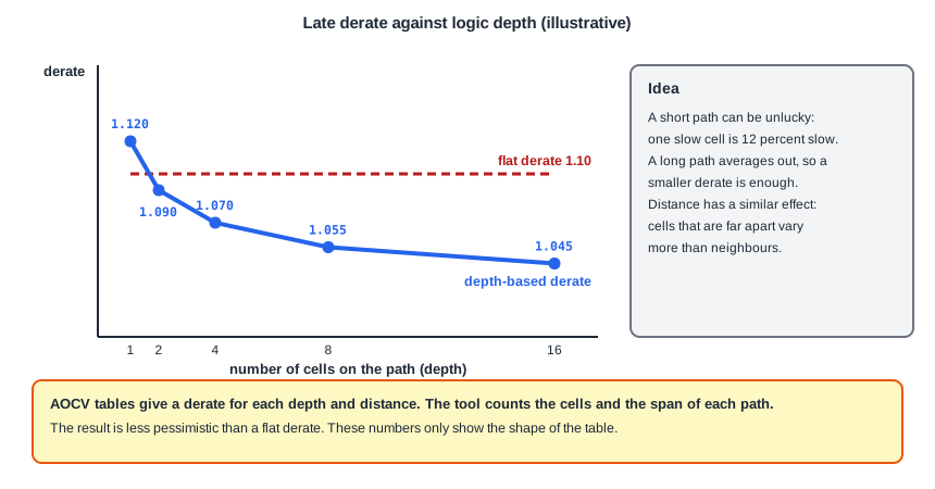
This is an illustrative table for the late derate:
| Depth (cells) | 1 | 2 | 4 | 8 | 16 |
|---|---|---|---|---|---|
| Late derate | 1.120 | 1.090 | 1.070 | 1.055 | 1.045 |
The tool counts the cells on each path and looks up the derate for that depth. Values between the entries are interpolated. A path of six cells gets a derate between the values for 4 and 8. The early derate has a similar table with values below 1.
Distance-Based Derating
There is a second effect. Cells that are close to each other vary in a similar way, because they see about the same process and temperature. Cells that are far apart vary more independently. For a path that spans a larger area of the chip, the variations are larger. AOCV tables have therefore a second axis, the distance, usually the size of the bounding box that holds the cells of the path. A derate table with depth and distance looks like this (illustrative):
| Depth \ Distance | 100 um | 500 um | 1000 um |
|---|---|---|---|
| 2 | 1.080 | 1.090 | 1.100 |
| 4 | 1.060 | 1.070 | 1.080 |
| 8 | 1.045 | 1.055 | 1.065 |
The derate grows with the distance and falls with the depth. A path of eight cells that stays within 100 micrometers has a late derate of 1.045. If it spans 1000 micrometers, it gets 1.065.
An Example
Take a data path of eight cells that has a nominal delay of 0.8 ns, which means 0.1 ns for each cell. The path stays within 500 micrometers. A flat late derate of 1.10 gives:
Flat derate:  0.800 x 1.10  = 0.880 ns
AOCV (depth 8, 500 um, 1.055):  0.800 x 1.055 = 0.844 ns
Margin given back: 0.880 - 0.844 = 0.036 ns
The setup slack of the path is 0.036 ns better with AOCV, on a single path. A design has thousands of critical paths, and this effect is often the difference between a design that can be closed and one that cannot. The result is still a pessimistic bound: AOCV does not say how likely the path is to be that slow, only that this is a reasonable worst case for its depth and size.
How It Is Used
- The AOCV tables come from the foundry or the library vendor and are read by the tool, in a separate file or in the library.
- The tool counts the depth and finds the bounding box of each path for the clock path and for the data path.
- Setup uses the late tables for the launch and data paths and the early tables for the capture path. Hold uses them the other way round, as for flat derates.
- The clock tree is a special case: the launch and capture paths share cells, so it is combined with the removal of common path pessimism.
The runs of this tutorial use flat derates, so the tables here are explained with arithmetic and not with a report.
Limits of AOCV
The depth and the distance are only two features of a path. The tables are built for typical cells, and a path with a few cells of very large variation is not described well. AOCV also needs a worst-case bounding box and cell count for each path, which takes run time. For these reasons, newer technologies use a statistical method that treats each cell separately. POCV and the Liberty Variation Format covers it.
Common Mistakes
Mistake #1: Using AOCV tables from a different technology or corner
The tables depend on the process and on the corner. Tables from another technology give a derate that does not match the real variation of your chip.
Mistake #2: Counting the depth of the wrong path
The depth is the number of cells on the path that is checked, not on the longest path of the design. Use the depth of the path in the report.
Quick Check: In an AOCV table, which is larger: the late derate of a path of 2 cells or of a path of 16 cells, at the same distance?
The path of 2 cells. The derate falls as the depth grows, because the random variations average out.
Practice Exercise
Challenge: Interpolate the Derate
This is a pencil and paper exercise with the illustrative depth table above. A path has 6 cells and a nominal delay of 0.6 ns. Find the late derate for 6 cells by linear interpolation between 4 and 8 cells. Then calculate the delay with AOCV and with a flat derate of 1.10.
Hint
Six is halfway between 4 and 8, so the derate is the mean of 1.070 and 1.055.
Solution
The derate is (1.070 + 1.055) / 2 = 1.0625. The AOCV delay is 0.6 x 1.0625 = 0.6375 ns and the flat delay is 0.6 x 1.10 = 0.660 ns. AOCV gives 0.0225 ns of margin back.
Summary
- A flat derate is the same for every path, and it is pessimistic for long paths because random variations average out.
- AOCV makes the derate depend on the number of cells on the path, which is the depth.
- It also depends on the distance spanned by the path, because far-apart cells vary more independently.
- The derate falls with the depth and grows with the distance.
- Setup uses the late tables for launch and data, and the early tables for capture. Hold is the other way round.
- The tables in this article are illustrative. Real tables come from the foundry.