CCS and ECSM

NLDM tables work well, but they rest on one simplification: the load of a cell is a single capacitor. In a real chip, the output of a cell drives a wire, and a wire has resistance as well as capacitance. For long or thin wires in small process nodes, this simplification costs accuracy. Current source models, called CCS and ECSM, were created to fix this. This article explains the problem and the idea behind the solution, without the full detail of the formats.

Think of filling a bucket through a long, thin hose. The tap sees a small load at first, because the water has not reached the far end yet. NLDM pretends the bucket is right at the tap. For short hoses that is fine, and for long thin ones it is not. Current source models describe the tap more carefully so that the hose can be taken into account.

6 min read | Intermediate

What You'll Learn

• Explain the assumption that NLDM makes about the load of a cell
• Describe what a current source model stores and how it differs from NLDM
• Name the extra data a CCS library adds: receiver capacitance and output current
• Check which delay model a library uses, and what that means for the lab

What NLDM Assumes

An NLDM table gives the delay for a given input slew and a given output capacitance. The cell is modeled as a driver charging one lumped capacitor.

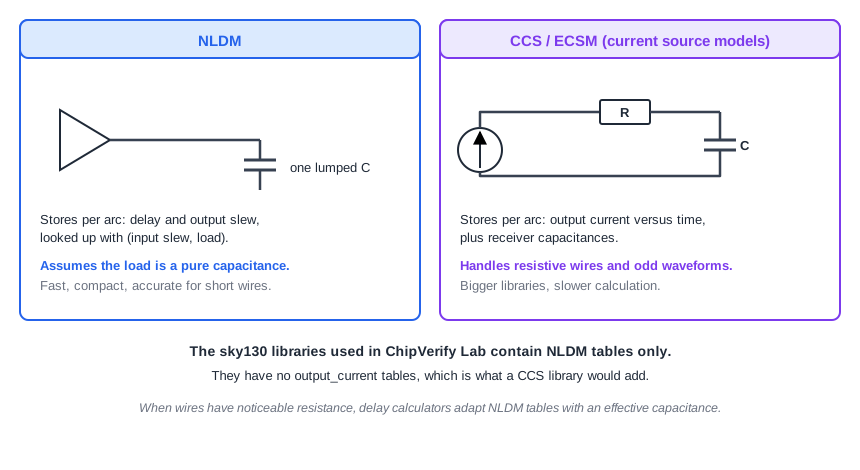
That is exact for a net that behaves like a single capacitor, such as a short wire. When the wire has noticeable resistance, the capacitance is spread along it, and the far end charges later than the near end. The cell no longer sees one capacitor.

Delay calculators handle moderate cases by finding an effective capacitance: one capacitor value that gives the same delay at the output of the cell as the real resistive net would. They then look up that value in the NLDM tables. A later chapter covers it. As process nodes shrink and wire resistance grows, the waveforms become more irregular, and this approximation loses accuracy.

The Idea of a Current Source Model

Instead of storing the final delay, current source models store how the output stage of the cell behaves. The output of a gate is modeled as a current source that charges whatever is connected to it. The tool can then drive the actual wire network with that current and compute the voltage waveform at every point, with the resistance included.

The two best-known models are:

• CCS, the Composite Current Source model
• ECSM, the Effective Current Source Model

Both follow the same idea, a time-varying, voltage-dependent current source for the output driver, with different file formats and details. In the rest of this article we use CCS as the example.

What a CCS Library Adds

A CCS library keeps the NLDM tables and adds two kinds of data.

• Receiver pin capacitance. In NLDM, an input pin has one capacitance value, or one for rising and one for falling. In CCS, the capacitance can differ between the first part and the last part of the transition, because the input stage of a cell does not act as a constant capacitor. The library has four tables: receiver_capacitance1_rise, receiver_capacitance1_fall, receiver_capacitance2_rise and receiver_capacitance2_fall.
• Output current. For each arc, and for each combination of input slew and output load, the library stores a waveform: the output current as a function of time. A group such as output_current_fall contains these waveforms.

output_current_fall () {
  vector ("template_name") {
    reference_time : ...;     /* when the input crosses its threshold */
    index_1(...);             /* input transition, one value */
    index_2(...);             /* output capacitance, one value */
    index_3(...);             /* time points */
    values(...);              /* output current at each time point */
  }
  ...  /* one vector for each combination of slew and load */
}

The waveforms need many points for every arc, so a CCS library is much larger than an NLDM library of the same cells, and the tool needs more calculation per arc. The gain is accuracy for resistive wires and unusual waveform shapes.

Which Model Does the Lab Use?

You can tell from the library. The header line delay_model : "table_lookup" means NLDM tables. A CCS library also contains output_current_rise and output_current_fall groups. The sky130 libraries of ChipVerify Lab have none of them, so every delay in the lab is an NLDM lookup. That fits the lab's pre-layout analysis, where the nets have no resistance at all and a lumped capacitor is exactly right.

The NLDM Table Edge

NLDM tables are only characterized up to a certain load. For the OR gate used on the path to z, the largest column is 0.1007 pF, which is also the max_capacitance of its output. A load heavier than that is outside the characterized range, and the tool has to extend the table beyond its last point. Even inside the table, delay and slew rise steeply for a weak cell. The exercise below pushes the cell toward this edge.

Common Mistakes

set_load 0.02 [get_ports z]
set_load 0.05 [get_ports z]
set_load 0.1 [get_ports z]