NLDM Delay Tables

The delay of a cell is not one number. The same AND gate is faster with a light load and slower with a heavy one, and faster when its input switches sharply than when the input is slow. Libraries capture this with lookup tables called NLDM, the Non-Linear Delay Model. This article shows how to read one and how the tool turns it into the delay you see in a report.

Think of filling a bucket from a tap. A bigger bucket takes longer to fill, and a tap that is turned on slowly delays everything further. A gate behaves in the same way: the bucket is the load on its output, and the speed at which the tap opens is the sharpness of its input edge. The table simply lists the answer for many combinations of the two.

8 min read | Intermediate

What You'll Learn

• Explain what the delay and output slew of a cell depend on
• Read an NLDM table: its two axes and its entries
• Calculate a delay by interpolating between table entries
• Describe how a cell changes the slew of the signal passing through it

Two Things That Set the Delay

A cell has to charge or discharge whatever its output is connected to, which is called the load. The delay depends on two factors:

• The output load: the capacitance on the output pin. A bigger capacitance takes longer to charge.
• The input slew: how long the input signal takes to change from low to high or from high to low. A slow input makes the cell switch later.

The output slew depends mainly on the load. A heavy load gives a slow output edge, and a slow input edge usually (not always) gives a larger delay. The slew of one cell's output is the input slew of the next cell, so slew travels along the path together with the delay.

The simplest model would be a formula, such as delay = D0 + D1 x slew + D2 x load. For modern cells a straight line is not accurate enough, so libraries store tables instead.

Reading an NLDM Table

Every arc has four tables: cell_rise and cell_fall for the delay of a rising and a falling output, and rise_transition and fall_transition for the output slew. Each table is a grid:

• The rows are indexed by the input slew (input_net_transition, index_1, in ns).
• The columns are indexed by the output load (total_output_net_capacitance, index_2, in pF).
• Each entry is the delay, or the output slew, in ns.

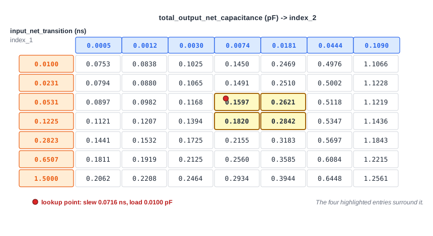
This is the cell_rise table of the arc from A to X of the and2_0 cell. Read it from left to right: with the sharpest input (0.0100 ns), the delay grows from 0.0753 ns at the lightest load to 1.1066 ns at the heaviest. Read it from top to bottom: at a fixed load, a slower input gives a larger delay.

Interpolation

A table only has values at its grid points. A real path hardly ever lands exactly on one, so the tool interpolates between the four nearest entries.

The path from the flip-flop _7_ through the AND gate to the output y has a rising input slew of 0.0716 ns at the AND gate. After set_load 0.01 on y, the load is 0.0100 pF. Both values fall between grid points, and the four highlighted entries surround them. The tool interpolates along the load first, then along the slew:

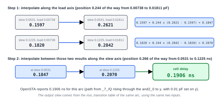
The hand calculation gives 0.1906 ns, and the timing report shows the same value:

             0.0716    0.0000    0.3058 ^ _3_/A (sky130_fd_sc_hd__and2_0)
   0.0100    0.1527    0.1906    0.4965 ^ _3_/X (sky130_fd_sc_hd__and2_0)

The first row shows the input slew 0.0716. The second shows the load 0.0100, the output slew 0.1527 and the delay 0.1906. The slew comes from the rise_transition table by the same interpolation.

A Cell Cleans Up a Slow Edge

The output slew of a cell depends mainly on its load, not on how slow its input was. This is why a cell can restore a poor signal. The AND gate on the path from input b shows it. With a sharp input (slew 0.0 ns) its delay is 0.1201 ns. With a very slow input (slew 0.3 ns) the delay more than doubles to 0.2537 ns, yet the output slew hardly changes:

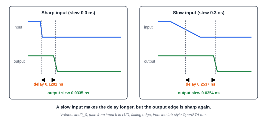
The delay grows with the input slew, but the output edge is sharp again, so only the delay of that one cell is affected, not every cell after it.

How the Numbers Are Measured

The header of the library fixes where on the waveform times and slews are measured. In the sky130 libraries, delay is measured between the 50% points of the input and the output. Slew is the time to go from 20% to 80% of the supply voltage, and the library applies no scaling to it (a derating factor of 1.0). Some other libraries measure slew between 10% and 90%, or between 30% and 70% and scale the result. Slews from libraries with different measurement points cannot be compared directly.

Common Mistakes

set_load 0.01 [get_ports y]