
A timing number at the end of synthesis is a prediction. The number at sign-off is the result. The two are never the same. The difference between them is the correlation problem, and a team that does not understand it keeps fixing the wrong paths, or finds out too late that the design is a long way from meeting timing. This article compares the same path at several levels of detail with real numbers, explains where the differences come from, and says what to do about them.
8 min read | Intermediate
What You'll Learn
- Define correlation between two timing runs
- Name the main reasons why pre-layout and post-layout timing differ
- Read the size of each effect from the demo circuit
- Describe how teams keep the early numbers close to the final ones
One Path at Several Levels
Take the path from the first to the second flip-flop of the demo circuit, with a 2.0 ns clock. This is the setup slack at the levels of detail that were used in the earlier articles:
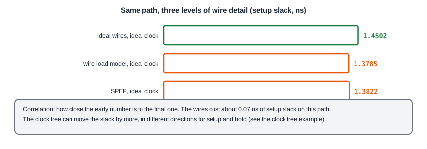
| Level of detail | Setup slack (ns) | Hold slack (ns) |
|---|---|---|
| ideal wires, ideal clocks | 1.4502 | 0.4241 |
| wire load model, ideal clocks | 1.3785 | 0.5072 |
| extracted wires (SPEF), ideal clocks | 1.3822 | 0.5129 |
The wires cost about 0.07 ns of setup slack, from 1.4502 ns to about 1.38 ns. The wire load model and the SPEF are close to each other, 1.3785 ns and 1.3822 ns, but this is a coincidence of this net: the model assumed 0.0060 pF and the SPEF has 0.0090 pF and an extra delay inside the wire. On another net, the two can differ a lot in either direction. The wires make the data slower, so the hold slack goes up by 0.08 ns, the opposite direction.
The clock tree is a second source. In the clock tree example of the article about clock latency, the path between the two flip-flops has a setup slack of 1.6889 ns and a hold slack of 0.2444 ns with a propagated clock, compared with 1.6200 ns and 0.3096 ns with ideal clocks. The skew of the real tree helps setup and hurts hold. For another path the skew goes the other way. The slack of a path can move by more than the effect of all the wires together.
Why the Numbers Differ
- Wires: the wire load model is a statistical guess, as the article about wire load models showed, and the real wires depend on the placement and the routing.
- Clocks: ideal clocks have no skew. The real clock tree has skew and latency, and both change slack.
- Crosstalk: neighbours add or remove delay, as in the chapter about signal integrity. It does not exist before routing.
- Variation: derates and the corners are usually added at the end.
- Optimizations: the placement and routing tools resize cells and insert buffers, which changes the paths.
- Constraints: a pre-layout run often uses simpler constraints.
What Correlation Means
Two runs correlate when the second is predictable from the first. A good correlation does not mean that the numbers are equal, but that the difference is small and similar for all paths. If the final slack is always about 0.07 ns lower than the early slack, a margin of 0.07 ns closes the gap. If some paths are 0.01 ns off and others 0.5 ns, the early run cannot be used to decide what to fix. Teams measure the correlation by plotting the post-layout slack against the pre-layout slack for all endpoints. A narrow cloud along a line is good. A wide cloud means that something is missing in the early run.
How Teams Keep Them Close
- A margin in the early runs: a clock uncertainty or a faster clock in synthesis that covers the expected effect of the wires and the clock tree.
- A better wire model: wire load models that are built from the results of earlier projects in the same technology, or a quick placement and a quick extraction instead of a model.
- Physical synthesis: synthesis tools that place the cells and use the real distances, so that the wires are not a guess.
- Early clock estimates: a latency or a skew on the ideal clock that represents the expected tree.
- Feeding back: after each project the differences are measured and the margins are adjusted.
What to Do With a Large Gap
If a path is much worse after layout, find the cause in the report: a long wire with a large net delay, a heavy load on a cell, a clock skew that hurts, or a crosstalk delay. Each cause has its own fix: a buffer, a stronger cell, a change of the clock tree, or more space. The reports of the post-layout run show the net delays and the clock paths that the pre-layout run did not have, so they point to the cause.
Common Mistakes
Mistake #1: Optimizing hard on pre-layout numbers
Paths that look critical early may not be critical at the end, and the reverse. Over-optimizing the early critical paths costs area for no gain.
Mistake #2: Looking only at setup
Wires and the clock tree change hold as well, and the direction is the opposite. A design that looks safe for hold before layout can fail after the clock tree is built.
Quick Check: A path has a pre-layout setup slack of 0.30 ns. After layout the slack is 0.12 ns. What is the correlation gap of this path?
0.30 - 0.12 = 0.18 ns, in the pessimistic direction.
Practice Exercise
Challenge: Measure the Gap
Use the sta_demo design. Note the setup slack of the path from _7_ to _6_ with ideal wires (1.4502 ns). Emulate a wire estimate by adding the wire load of the example model with set_load:
set_load 0.006 [get_nets r1]
set_load 0.004 [get_nets _1_]
Predict the setup slack and the hold slack of the same path, and calculate the gap in both checks compared with the ideal wires.
Open the ready-made example in the lab, run synthesis, and then run STA. Editing constraints.sdc and re-running only STA, and choosing another library or corner, are PRO features.
Hint
The article about wire load models gives the result of exactly these two commands. Wires make the data slower, so setup falls and hold rises.
Solution
The setup slack is 1.3785 ns, a gap of 1.4502 - 1.3785 = 0.0717 ns. The hold slack is 0.5072 ns, which is 0.5072 - 0.4241 = 0.0831 ns higher. The two gaps have opposite signs, so a margin for the wires helps setup and has to be applied carefully for hold.
Summary
- Timing before layout is a prediction, and timing after layout is the result. The difference is the correlation gap.
- On the demo path, wires lower the setup slack by about 0.07 ns and raise the hold slack by about 0.08 ns.
- The clock tree can change slack by as much as all the wires together, and in the opposite direction for setup and hold.
- Crosstalk, variation and optimization add more differences later in the flow.
- A good correlation means that the gap is small and similar for all paths.
- Teams use margins, better wire models, physical synthesis and early clock estimates to close the gap, and they measure it after every project.
