
AOCV improves the flat derate by looking at the depth and the distance of a path. It still uses one number for a whole path. Parametric OCV, POCV, which is also called statistical OCV, goes one step further. It describes the variation of every cell with a standard deviation, and it adds the variations of the cells on a path in a statistical way. The data for this lives in the library, in a format called the Liberty Variation Format, LVF. This article explains the idea, the arithmetic, and how the library carries the numbers. The numbers in the examples are made up to show the method.
9 min read | Intermediate
What You'll Learn
- Explain what a standard deviation of a cell delay means
- Combine the variations of the cells of a path with the root of the sum of squares
- Compare the statistical margin with a flat derate for short and long paths
- Describe what the Liberty Variation Format adds to a library
Each Cell Has a Mean and a Sigma
In the libraries that you have seen so far, a cell arc has one delay for each combination of input slew and load. A cell with variation data has two numbers for each combination: the mean delay, which is the same number as before, and the standard deviation of the delay, written sigma. Sigma is a measure of the spread of the delay between chips. About two thirds of the chips have a delay within one sigma of the mean, and nearly all of them, 99.7 percent, within three sigma.
A cell with a mean delay of 0.100 ns and a sigma of 0.010 ns has a delay of 0.100 ns plus or minus 0.010 ns for most chips, and it is between 0.070 and 0.130 ns for almost all of them.
Adding Cells on a Path
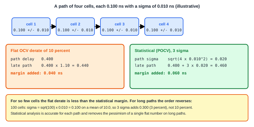
The means add up in the usual way: a path of four cells with 0.100 ns each has a mean of 0.400 ns. The sigmas do not add up in the same way. If the variations of the cells are independent, the variance, which is sigma squared, adds up:
path sigma = sqrt( sigma1^2 + sigma2^2 + sigma3^2 + sigma4^2 )
           = sqrt( 4 x 0.010^2 ) = 0.020 ns
The sigma of the path is 0.020 ns, and not 4 x 0.010 = 0.040 ns. The path is less uncertain than the sum of the cells, because slow and fast cells compensate each other. For a path of N equal cells, the sigma of the path grows with the square root of N, while the mean grows with N. The relative spread falls as the path gets longer.
The Margin
For the check, STA uses the mean plus a number of sigmas for the late delays and the mean minus the same number for the early delays. A common choice is three sigma:
| Method | Late delay of the 4-cell path | Margin added |
|---|---|---|
| Flat derate 1.10 | 0.400 x 1.10 = 0.440 ns | 0.040 ns |
| 3 sigma statistical | 0.400 + 3 x 0.020 = 0.460 ns | 0.060 ns |
For this short path the statistical margin is larger than the flat derate. For a long path, it is much smaller. A path of 100 cells of 0.100 ns each has a mean of 10.0 ns and a sigma of sqrt(100) x 0.010 = 0.100 ns. Three sigma add 0.300 ns, which is 3 percent. A flat derate of 10 percent would add 1.0 ns. This is the main benefit of the statistical method: it is accurate for each path. The margin is large where the path is short and the variation is large compared with the mean, and small where the averaging helps.
Where the Numbers Come From: LVF
The library has to supply the sigma of every cell arc, for every combination of slew and load. The Liberty Variation Format adds tables to the timing groups for this. They have the same two axes as the delay tables. The names of the main ones are:
ocv_sigma_cell_riseandocv_sigma_cell_fall: the standard deviation of the cell delay for a rising and a falling output.ocv_sigma_rise_transitionandocv_sigma_fall_transition: the standard deviation of the output slew.- The setup and hold constraint tables also have sigma tables, so that the check itself has a spread.
The tables can come in an early and a late form, because the distribution of a delay is not always symmetric: the slow side can be longer than the fast side. A table is marked with an attribute that says if it is for early values, for late values, or for both.
The sky130 libraries used in this tutorial have no variation tables. A search for the sigma tables in the three corner libraries finds none, so the numbers in this article are examples and not results of a run.
Strengths and Limits
- The method is accurate per path and it removes the large pessimism of flat derates on long paths.
- It needs the sigma data for the whole library, which is expensive to produce, because each arc is simulated many times with random variation.
- The simple root of the sum of squares assumes that the cells vary independently. A part of the variation is shared between neighbouring cells, and a good tool treats it separately.
- The wires are often handled with a flat derate, because the library data only covers cells.
- The number of sigmas is a choice. More sigmas give a safer chip and a more pessimistic report.
Common Mistakes
Mistake #1: Adding sigmas linearly
The sigma of a path is the root of the sum of the squares, not the sum. Adding sigmas gives a margin that is far too large for a long path.
Mistake #2: Comparing a flat derate and a statistical margin on one path
On a short path the statistical margin can be larger than the flat derate. The advantage appears on the long paths, and the comparison has to be made over the whole design.
Quick Check: A path has 9 equal cells, each with a sigma of 0.02 ns. What is the sigma of the path?
sqrt(9 x 0.02^2) = 3 x 0.02 = 0.06 ns.
Practice Exercise
Challenge: Statistical or Flat?
This is a pencil and paper exercise. A path has 25 cells with a mean delay of 0.080 ns and a sigma of 0.008 ns each. Calculate the late delay with a 3 sigma statistical margin and with a flat derate of 1.10, and say which is more pessimistic.
Hint
The mean of the path is 25 x 0.080. The sigma of the path is sqrt(25) x 0.008.
Solution
The mean is 2.000 ns and the sigma is 5 x 0.008 = 0.040 ns. The statistical late delay is 2.000 + 3 x 0.040 = 2.120 ns, and the flat late delay is 2.000 x 1.10 = 2.200 ns. The flat derate is more pessimistic by 0.080 ns. For a path of 4 cells, the order would be the other way round, as in the example above.
Summary
- POCV gives every cell a mean delay and a standard deviation, sigma, and adds them along the path.
- The means add linearly. The sigmas add as the root of the sum of squares.
- The late delay is the mean plus a number of sigmas, often three, and the early delay is the mean minus them.
- For short paths the statistical margin can be larger than a flat derate, and for long paths it is much smaller.
- The Liberty Variation Format carries the sigma tables, such as
ocv_sigma_cell_rise, in the library. - The sky130 libraries of this tutorial have no variation data, so the examples are calculated by hand.
