
Post-silicon learning does not stop at release. Yield data shows what fraction of parts work and why the rest do not, and field returns show what escaped every test. Both feed improvements to the process, the test program and the next design.
This article covers the main kinds of yield loss, a simple yield model, and how returned parts are analysed.
6 min read | Intermediate
What You'll Learn
- Distinguish defect-limited and parametric yield loss
- Use a simple model to relate die area and defect density to yield
- Follow a field return through analysis
- Explain how returns improve test and design
Yield and Its Losses
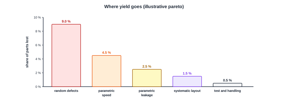
Yield is the fraction of parts that pass all tests. The losses fall into broad groups:
- Defect-limited: random particles and flaws break some die.
- Parametric: die work but miss speed, power or leakage limits, the subject of Fmax and Binning.
- Systematic: a layout pattern that the process prints poorly fails on many die in the same place.
- Test and handling: good parts lost to test errors or damage.
A pareto of loss causes shows where effort pays most. Wafer maps help separate random defects from systematic patterns, as in Characterizing Many Parts.
A Simple Yield Model
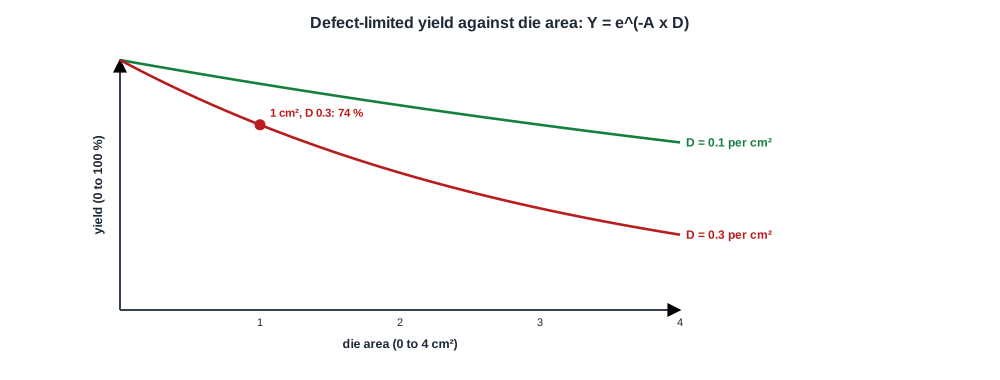
For random defects spread evenly, a common first approximation is Y = e-A x D, where A is the die area and D the defect density. Bigger die and dirtier processes both lower yield.
Quick Check
Q: A 1 cm2 die in a process with 0.2 defects per cm2. What is the defect-limited yield? What if the die were 2 cm2?
Show Answer
e-0.2 is about 82 %. At 2 cm2, e-0.4 is about 67 %. Doubling the area lowers yield and also halves the number of die per wafer, so cost per good die rises sharply.
Field Returns
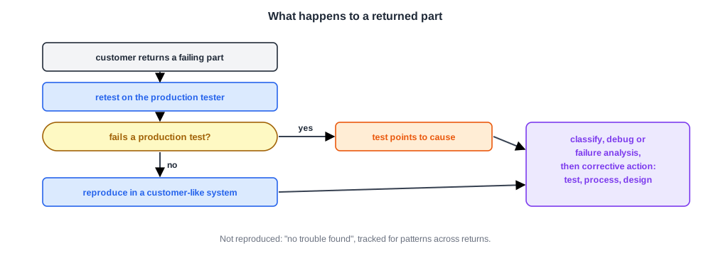
- Retest: the part runs the production test program. If it fails, the failing test points to the problem.
- System reproduction: if it passes, engineers try to reproduce the failure in a system like the customer's. Many returns end as "no trouble found".
- Classification and analysis: as in Classifying Failures, then debug or physical failure analysis.
- Corrective action: a new test or tighter limit, a process change, an erratum, or a design change for the next product.
Debug features are essential here, which is why locked parts need an authenticated way back in, as described in Locking Debug.
Quick Check
Q: A returned part passes every production test and works in the lab system. What should still be done?
Show Answer
Look for the customer's conditions: temperature, voltage, workload, board and firmware. Track it with similar returns, since a pattern across several "no trouble found" parts often reveals a real escape that only appears under specific conditions.
In Practice
Yield and return data are reviewed regularly across product, test, process and design teams. Each confirmed escape gets a test, each systematic yield loss a process or layout fix, and lessons go into the design rules and validation plan of the next chip.
Common Mistakes
Mistake #1: Treating all yield loss as random defects
Separate parametric and systematic loss; they need different fixes.
Mistake #2: Closing "no trouble found" returns without follow-up
Patterns across returns often reveal real escapes.
Mistake #3: Fixing returns only in test
Feed lessons into the next design and validation plan too.
Practice Exercise
Challenge: Cost per Good Die
A wafer holds 600 die of 1 cm2. Defect density is 0.3 per cm2, and a wafer costs 6,000 units.
What is the cost per good die? If process improvements lower the density to 0.15, what is it then? Use Y = e-A x D.
Hint
Good die = 600 x Y.
Solution
Y = e-0.3 = 0.74, so 444 good die and about 13.5 per die. At 0.15, Y = e-0.15 = 0.86, 516 good die, about 11.6 per die: a 14 % cost reduction from yield learning alone.
Summary
- Yield loss is defect-limited, parametric, systematic, or from test and handling.
- A simple model Y = e-A x D shows how area and defect density drive yield.
- Field returns are retested, reproduced, classified and analysed to find escapes.
- Corrective actions improve test, process and the next design.
