SystemVerilog solve before

The SystemVerilog constraint solver by default tries to give a uniform distribution of random values. Hence the probability of any legal value of being a solution to a given constraint is the same.

But the use of solve - before can change the distribution of probability such that certain corner cases can be forced to be chosen more often than others. We'll see the effect of solve - before by comparing an example with and without the use of this construct.

Random Distribution Example

For example, consider the example below where a 3-bit random variable b can have 8 legal values ( 2³ combinations). The probability of b getting a value 0 is the same as that of all other possible values.

class ABC;
	rand bit [2:0]  b;
endclass

module tb;
	initial begin
		ABC abc = new;
		for (int i = 0; i < 10; i++) begin
			abc.randomize();
			$display ("b=%0d", abc.b);
		end
	end
endmodule

Note that even though there are repeated values in the simulation output shown below, it only means that a previous randomization had no effect on the current iteration. Hence the randomizer is free to pick any of the 8 values regardless of what the previous value was.

ncsim> run
b=7
b=7
b=2
b=1
b=6
b=4
b=2
b=4
b=0
b=1
ncsim: *W,RNQUIE: Simulation is complete.

However, the probability that any of the 8 legal values becoming a solution is the same for all values.

Without solve - before

Consider the following example shown below where two random variables are declared. The constraint ensures that b gets 0x3 whenever a is 1.

class ABC;
  rand  bit			a;
  rand  bit [1:0] 	b;
  
  constraint c_ab { a -> b == 3'h3; }
endclass

module tb;
  initial begin
    ABC abc = new;
    for (int i = 0; i < 8; i++) begin
      abc.randomize();
      $display ("a=%0d b=%0d", abc.a, abc.b);
    end
  end
endmodule

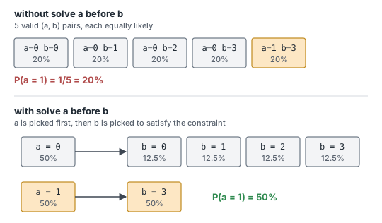
Note that a and b are determined together and not one after the other.

ncsim> run
a=0 b=0
a=0 b=1
a=0 b=0
a=0 b=1
a=0 b=2
a=1 b=3
a=0 b=3
a=0 b=3
ncsim: *W,RNQUIE: Simulation is complete.

When a is 0, b can take any of the 4 values. So there are 4 combinations here. Next when a is 1, b can take only 1 value and so there is only 1 combination possible.

Hence there are 5 possible combinations and if the constraint solver has to allot each an equal probability, the probability to pick any of the combination is 1/5.

With solve - before

SystemVerilog allows a mechanism to order variables so that a can be chosen independently of b. This is done using solve keyword.

class ABC;
  rand  bit			a;
  rand  bit [1:0] 	b;
  
  constraint c_ab { a -> b == 3'h3; 
  				
  				  // Tells the solver that "a" has
  				  // to be solved before attempting "b"
  				  // Hence value of "a" determines value 
  				  // of "b" here
                  	solve a before b;
                  }
endclass

module tb;
  initial begin
    ABC abc = new;
    for (int i = 0; i < 8; i++) begin
      abc.randomize();
      $display ("a=%0d b=%0d", abc.a, abc.b);
    end
  end
endmodule

Compare this output with the previous one to see the difference. Here, a is solved first and based on what it gets b is solved next.

ncsim> run
a=1 b=3
a=1 b=3
a=0 b=1
a=0 b=0
a=0 b=0
a=0 b=1
a=1 b=3
a=0 b=2
ncsim: *W,RNQUIE: Simulation is complete.

Because a is solved first, the probability of choosing either 0 or 1 is 50%. Next, the probability of choosing a value for b depends on the value chosen for a.

Note that the probability of b is almost 0% before and after using solve - before, it has become a little more than 50%.

Restrictions

There are a few restrictions in the use of solve before which are listed down below.

• randc variables are not allowed since they are always solved first
• Variables should be integral values
• There should not be circular dependency in the ordering such as solve a before b combined with solve b before a.