Predictor Accuracy and Sizing

How large should a branch predictor be? More storage usually means better accuracy, but with sharply diminishing returns, and at some point the extra area would do more good elsewhere. The way to answer is a sizing study: run real branch traces through models of different sizes, turn the accuracy into performance, and compare it with the cost. This article shows how such a study works, runs one on six small programs, and draws out what it can and cannot prove.

12 min read | Intermediate

What You'll Learn

• Describe how a trace-driven predictor study works
• Read accuracy and mispredictions per kilo-instruction correctly
• Turn a predictor's accuracy into a gain in CPI
• Decide when a larger predictor stops being worth its area

How a Study Works

A detailed simulation of a whole processor is slow, and a predictor can be studied without one. A trace-driven model needs only a list of the branches a program executed, in order: each branch's address, whether it was taken, and its target. A short script then feeds that list to a software model of each predictor, one branch at a time. It looks up the prediction, compares it with the recorded outcome, and updates the table.

That takes seconds rather than days, so dozens of sizes and designs can be compared. The trace in this article was recorded by running six small compiled RV32I programs in a simple simulator. Its counts of instructions, loads and branches matched a real five-stage processor design exactly, so the traces can be trusted to show what the programs do. The script is only about two hundred lines, and writing one is a good way to get a feel for how these structures behave.

A trace-driven model has limits. It sees only the correct path, never the wrong-path instructions, and it updates each table at once, not many cycles later as real hardware does. For a large core, both effects matter, and final numbers come from a detailed simulator. For choosing a size, a trace is usually good enough.

Measuring Accuracy Well

Accuracy is the fraction of branches predicted correctly. It is easy to understand, but it hides how often branches occur. Engineers therefore usually report MPKI, mispredictions per kilo-instruction, the number of wrong predictions per 1,000 executed instructions:

MPKI = branches per instruction x (1 - accuracy) x 1,000

MPKI connects directly to performance, because the cycles lost per instruction are MPKI / 1,000 x penalty. A program with a branch every 5 instructions at 95 percent accuracy has an MPKI of 10. On a 15-cycle penalty, that loses 0.15 cycles per instruction. Good large-core predictors reach an MPKI of a few or less on typical integer programs, though some programs stay stubbornly higher.

The Study

Bimodal and gshare predictors with 16, 64, 256, 1,024 and 4,096 two-bit counters were run on each trace. For gshare, the history length matched the index width. Dynamic Predictors: Bimodal and gshare explains both designs. Here are three of the programs:

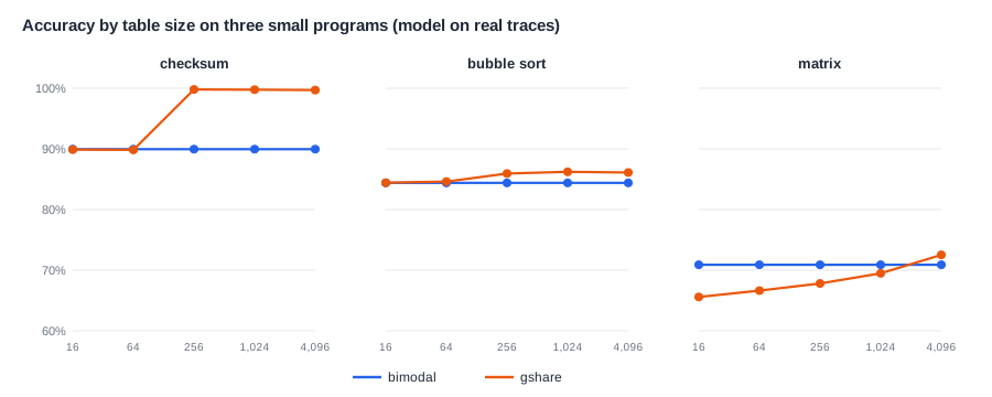
Each chart tells a different story.

Bimodal is flat. On all three programs, 16 counters do as well as 4,096. These programs have so few branches in their loops that even a tiny table holds them all. Only the linked-list program, with more branches in its code, showed any gain, and that was less than a percentage point from 16 to 256 entries. Bigger software would need a bigger table, but the shape is the same: accuracy rises until each active branch has its own counter, and then it stops.

gshare depends on the table. On the checksum it jumps from 90 to 99.8 percent when the table reaches 256 entries, because then the history is long enough to span the whole inner loop. A shorter history simply cannot see the pattern. On the matrix program it starts well below bimodal at small sizes, and it only passes bimodal at the largest size, because each branch is spread over many counters that interfere with each other.

Some programs do not care. The bubble sort stays near 85 percent whatever the size or design, because its hard branch depends on random data. No table can learn that.

From Accuracy to Performance

A chart of accuracy can mislead, so turn it into CPI. The processor is a simple five-stage core where a wrong guess costs 2 cycles, and a correctly predicted taken branch is assumed to cost nothing, thanks to a branch target buffer. Without any predictor, the programs had a CPI of up to about 1.6. For the linked-list program, predicting not taken loses about a third of its cycles to flushes. With 256 bimodal counters, its CPI falls from about 1.5 to about 1.1, a speedup of about 1.35. For a matrix program it falls from about 1.45 to about 1.17, a speedup of about 1.25.

Even a tiny predictor gives a large gain, because the first step, from always guessing not taken on a loop, is the biggest. Moving on from 256 to 4,096 counters on this small core gives almost nothing, since each mistake costs only 2 cycles. On a large core with a 15-cycle penalty, the same small gain in accuracy is worth far more. That is why predictor size follows pipeline depth.

Weighing the Cost

A two-bit table is small. 256 counters take 64 bytes, and 4,096 take 1 KB. Storage in a predictor is not free, though. It must be read every cycle, in the fetch stage, within a tight time limit, and it burns power on every read and update. The rough steps of a decision look like this:

1. Measure the MPKI on real workloads for several sizes.
2. Multiply by the design's penalty to get lost CPI.
3. Compare the gain with the area, using PPA Trade-offs and Amdahl's Law.
4. Check the access time, since a table too slow for one cycle costs a cycle on every taken branch.
5. Stop where a doubling in size no longer pays for itself.

History Length Is a Second Dial

Table size is not the only setting. A gshare predictor also has a history length, and the two interact. In the study above, history length grew with the table, one bit per doubling. A longer history can see patterns further back, but each branch then uses more counters, so learning takes longer and the table fills up faster. For a fixed table, the best history length is usually shorter than the maximum.

The checksum shows why length can matter more than size. Its inner loop needs about eight bits of history to see the loop exit. With six bits, gshare stays at 90 percent however the bits are used. With eight, it goes straight to nearly perfect. A designer who tested only short histories would conclude, wrongly, that history is useless for this program. Modern predictors avoid having to choose. They keep several tables with different history lengths and let each branch use whichever length works for it.

Initial values are a smaller dial. Starting all counters at "weakly not taken" or "weakly taken" makes a small difference on long programs, but it can matter on very short ones, where warm-up is a large part of the run. On small embedded programs that run for moments and then sleep, a predictor may never really warm up at all.

What This Study Cannot Tell You

These six programs are tiny. A web browser or a database has hundreds of thousands of branch instructions, and many of them run rarely. There, aliasing is a real problem, tables never fill up with only the useful branches, and warm-up costs matter. A study on small kernels will always make a small table look enough. Workloads and Benchmarks explains why the choice of programs matters more than anything else in a study.

Context switches matter as well. When the operating system changes to another program, the tables are full of the old program's history, so the new one starts with a poorly trained predictor. And a large number of tasks, such as many threads on one core, can share and disturb the same tables.

Sometimes the best answer is outside the predictor. In one of the tests above, a program's branch mispredictions came mostly from a single multiply routine that tests one bit of its operand per pass. A hardware multiply instruction removes those branches altogether. Changing the instruction set or the code can beat any table, as ISA Design Choices discusses.

Build Your Own Study

A small study is easy to do on a PC. Compile a few C programs for a simple instruction set, and run them in a free instruction-set simulator that can print each branch. Or instrument the source code with a macro that records each if. A Python model of a two-bit table takes about twenty lines:

table = [1] * size                       # all counters start at weakly not taken
for pc, taken in trace:
    i = (pc >> 2) & (size - 1)           # drop the two low bits of the address
    correct += (table[i] >= 2) == taken
    table[i] = min(3, table[i] + 1) if taken else max(0, table[i] - 1)

Adding gshare takes only two more lines. The value of doing this yourself is that the results often surprise you, which is the real point of measuring.

Common Mistakes