
A performance model is a program that predicts how fast a processor will run, before the processor exists. Architects cannot build each idea in silicon, so they test them in models, ranging from a few formulas in a spreadsheet to detailed simulators that track every instruction. Each trades accuracy against speed, and the skill lies in choosing the right one. This article explains the kinds of model, builds a simple one that predicts the cycles of a real pipeline exactly, and shows how models are calibrated and how they mislead.
12 min read | Intermediate
What You'll Learn
- Compare analytical, trace-driven and cycle-accurate models
- Build a simple cycle model from a pipeline's stall and flush rules
- Explain calibration and how to judge a model's error
- Recognize when a model's conclusion should not be trusted
Why Model at All
Designing a processor takes years and costs a great deal, and most of the important decisions are made early, when there is no RTL. How wide? How large a cache? Is a new predictor worth its area? Answers can come only from a model. The aim is to find the shape of the design space cheaply, and to avoid building what doesn't help.
Every model trades three things against each other:
- Speed: how quickly it runs.
- Accuracy: how close it is to the real thing.
- Development effort: how long it takes to build, and to change.
Kinds of Model
From fastest to slowest:
| Model | Speed | Typical use |
|---|---|---|
| Analytical: formulas, spreadsheets | instant | early budgets, sanity checks |
| Functional simulator: runs instructions, with no timing | hundreds of millions of instructions per second | running software early, producing traces |
| Trace-driven: feeds a recorded trace to a model of one block | millions per second | cache and predictor studies |
| Cycle-accurate simulator, in C++ or similar | thousands to hundreds of thousands per second | full-core performance studies |
| RTL simulation | tens to thousands of cycles per second for a large design | final checks |
| FPGA or emulation | millions of cycles per second | running large software on the real design |
The performance equation is the simplest analytical model. The trace-driven kind appeared in Predictor Accuracy and Sizing and Cache Sizing Studies. Open-source cycle-level simulators such as gem5 are widely used in research, and companies build their own.
A Simple Model That Works
A simple pipeline is regular enough to be predicted by a few rules. Take a five-stage core with forwarding, in which every instruction takes one cycle, except for these costs:
cycles =  instructions
        + 2 x (taken branches + completed jumps)     flush cost
        + load-use stalls                            one per case
        + 4                                          filling the pipeline at the start
This needs only counts that a functional simulator can produce. It knows nothing about timing inside the core. Here is how the two estimates compare with a real RTL simulation of six small programs:
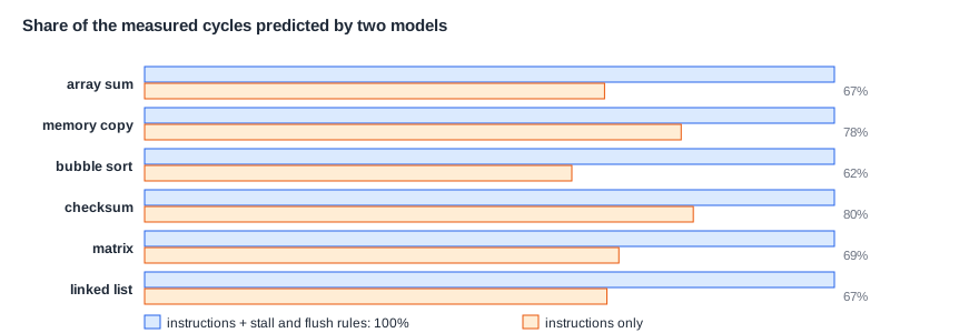
The rule-based model matched the measured cycle count exactly on all six programs. Counting instructions alone gives 62 to 80 percent of the real number: it misses a fifth to well over a third of the cycles. For a simple in-order core with a fast memory, a handful of rules captures the whole machine.
Such a perfect result is rare, and it should make you suspicious. It works here because the design is simple and the memory is ideal. With a real cache, the cost of a miss depends on what is in the cache, so the model needs a cache simulator. With a large core, costs overlap: two cache misses in flight together don't simply add up. The model then gets harder, and it is usually better to simulate.
Quick Check
Q: Using the formula above, what are the predicted cycles for 10,000 instructions, 1,500 taken branches, 200 completed jumps and 100 load-use stalls?
Show Answer
10,000 + 2 x 1,700 + 100 + 4 = 13,504 cycles, so a CPI of 1.35.
Interval Analysis
For out-of-order cores, there is a clever middle ground. A core runs smoothly at its peak rate, until something interrupts it, such as a branch misprediction or a long cache miss. Interval analysis treats a run as a series of such intervals. Between events, the IPC is near a steady value determined by the dependences in the program. Each miss event adds a penalty that can be estimated. With event counts from a trace, a spreadsheet model like this can get within about 10 percent of a detailed simulator, and it helps to explain why a program is slow.
The issue models shown in Out-of-Order Execution and Register Renaming are in the same family. They use the real dependences from a trace, and ignore many details, such as the front end and the memory. They give an upper limit rather than a prediction.
Building a Cycle-Accurate Simulator
A detailed simulator models each stage of the pipeline as a software object, advancing one simulated cycle at a time. Instructions flow through queues that behave like the real ones, with structural limits on each one. Two designs are common. Trace-driven simulators feed in a list of instructions and can't model wrong paths. Execution-driven simulators run the program, so they can model wrong-path work, and interactions between threads.
Long programs are too slow to simulate in full, so simulators use sampling: run fast through most of the program, and simulate in detail only in short slices. Methods such as SimPoint choose slices that represent the whole program, by looking at which code runs when. A few hundred million simulated instructions can stand for trillions of real ones.
Calibration
A model is only useful if it is right, so it must be compared with something real. Calibration means running small test programs on both a real machine, or RTL, and the model, and then fixing the differences. Small targeted tests, called microbenchmarks, measure one thing each: a load-to-use time, a branch penalty, a cache size. Once each is right, whole programs are compared.
The most useful result is a relative one. A model that is 10 percent off on absolute IPC may still predict correctly that a design change gives 3 percent, because the same error affects both runs. But watch out: when two options are within a percent or two of each other, the model's noise can decide the answer. Architects also keep track of a model's error over time, and improve the parts that matter most.
Where Is This Used?
A processor project usually has a performance team, separate from the RTL team, maintaining a detailed model throughout the project. Early on, it steers the architecture. Later, its predictions are compared with RTL runs, and a mismatch often exposes a performance bug in the RTL: a queue that's a bit too small, or a stall that shouldn't be there. Software teams use these models as well, to tune compilers before silicon exists. Datasheet performance targets usually come from such models, long before the first chip.
How Models Mislead
A model reflects what its authors thought was important. The most common failures are these:
- False precision. A result printed to four digits from a model with a 10 percent error means nothing past the first digit or so.
- The wrong workload. A small benchmark that fits in the cache hides memory problems, as Workloads and Benchmarks explains.
- Missing effects. A model that ignores the operating system, wrong-path work or prefetching can be badly off on real software.
- Tuning to the model. Optimizing a design against a model can exploit its flaws, like tuning to a benchmark.
- Ignoring physics. A model may make a queue larger at no cost, while in reality that queue would not fit in a cycle. Timing and power need to be checked as well.
A useful habit is to ask what would have to be true for the model to be wrong, and then to test that. Another is to predict a simple result by hand first. If the simulator disagrees with a calculation, one of them has a bug.
Quick Check
Q: A cycle-accurate model has a known error of about 5 percent on IPC. It reports that feature A gives a 1.5 percent gain. Should you trust the gain?
Show Answer
Possibly. If the error is similar with and without the feature, the difference can still be meaningful. But a 1.5 percent gain needs careful checks: test more workloads, and confirm that the effect is not an artifact of the model. Never compare it directly with the 5 percent figure.
A Worked Analytical Model
Even a spreadsheet can answer real questions, if it starts from measured event rates. Suppose a core with an ideal IPC of 2 runs a workload with 5 branch mispredictions and 3 L2 misses per 1,000 instructions, at a 15-cycle penalty and a 100-cycle penalty. These numbers are assumptions for this example. The cycles per 1,000 instructions are:
base:        1,000 / 2           =  500
branches:    5 x 15              =   75
L2 misses:   3 x 100             =  300
total                            =  875     IPC = 1,000 / 875 = 1.14
The result says at once that memory, not branches and not width, is the main loss. Doubling the width to give an ideal IPC of 4 takes the total to 625 cycles, a gain of 40 percent, which is optimistic, since it assumes the program has that parallelism. Halving the L2 misses takes it to 725 cycles, a gain of 21 percent, and probably for a lot less hardware. Ten minutes with these numbers can shape a project's direction, and show which questions a detailed simulator should answer next. This is the same reasoning as a CPI stack, used in reverse to look at options that don't exist yet.
Models for Power and Area
Performance is only one of the three PPA numbers, and models exist for the other two as well. Early power models attach an energy cost to each event, such as a cache access or an instruction decoded, and multiply by event counts from a simulator. Tools such as McPAT estimate power and area from a design's parameters. These are rougher than performance models, often only within 20 percent or so. Once RTL exists, synthesis gives much better figures, using real switching activity from a simulation, as PPA Trade-offs and Amdahl's Law discusses.
Models also age. One tuned for an earlier generation can carry assumptions that no longer hold, so teams check it again against each new chip when silicon arrives.
Power models need calibrating as well, against RTL power estimates and later against silicon. Without that, they show only trends.
Keep each model's assumptions written down next to its results, so that anyone reading a number later can judge how far to trust it.
Common Mistakes
Mistake #1: Using a model outside its calibrated range
A model tuned for small caches may be wrong for large ones. Recalibrate when the design moves far from what was validated.
Mistake #2: Reporting one number from one run
Random seeds, sampled slices and workloads all add variation. Report several runs and a range, particularly for small effects.
Mistake #3: Building detail before asking the question
A spreadsheet may answer in an hour what a simulator takes months to answer. Use the simplest model that can answer the question, and add detail only where the answer depends on it.
Practice Exercise
Challenge: Build and Use a Model
A five-stage core has these costs: 2 cycles per taken branch, 1 cycle per load-use stall, and 20 cycles per cache miss. These numbers are assumptions for this exercise. A program runs 1,000,000 instructions, with 120,000 taken branches, 30,000 load-use stalls and 8,000 cache misses. (a) Predict the cycles and the CPI. (b) A predictor removes 70 percent of the branch flushes. What is the new CPI? (c) A larger cache removes half of the misses. What is the new CPI? (d) A real run of the base design took 1,350,000 cycles. What is the model's error, and what might it be missing?
Hint
Add each cost to the instruction count. For (d), the error is (model - real) / real.
Solution
(a) 1,000,000 + 240,000 + 30,000 + 160,000 = 1,430,000 cycles, a CPI of 1.43. (b) Branches fall to 72,000: 1,262,000 cycles, a CPI of 1.26. (c) Misses fall to 80,000: 1,350,000 cycles, a CPI of 1.35. (d) (1,430,000 - 1,350,000) / 1,350,000 = 5.9 percent high. The model may overcount, for example if some misses overlap with branch flushes, or if the real miss penalty is shorter than 20 cycles on average.
Summary
- Models trade speed, accuracy and effort, from formulas up to cycle-accurate simulators.
- A few rules predicted a simple pipeline's cycles exactly on six programs, where instruction counts alone missed up to 38 percent.
- Sampling makes long programs possible to simulate.
- Calibrate against real hardware or RTL, and trust relative results more than absolute ones.
- Use the simplest model that answers the question, and look for what it leaves out.
