
A dynamic branch predictor learns from what each branch has done so far. The idea is simple: keep a small table of counters, and use the past to guess the future. A two-bit counter per branch handles loops well, and adding a record of recent branch outcomes lets the predictor catch patterns that no single counter can see. This article builds up from a single bit of memory to the bimodal predictor, explains aliasing and correlation, shows how gshare works, and then looks at what modern predictors add, with results from real branch traces.
12 min read | Intermediate
What You'll Learn
- Explain why a two-bit counter beats a one-bit memory on loops
- Describe how a bimodal predictor indexes its table and what aliasing does
- Explain how global history lets a predictor use correlation between branches
- Describe how gshare forms its index and when it beats bimodal
One Bit of Memory
The simplest learning predictor stores one bit for each branch: what the branch did last time. The prediction is "the same again". For a long loop this is nearly perfect, but look at what happens at each end:
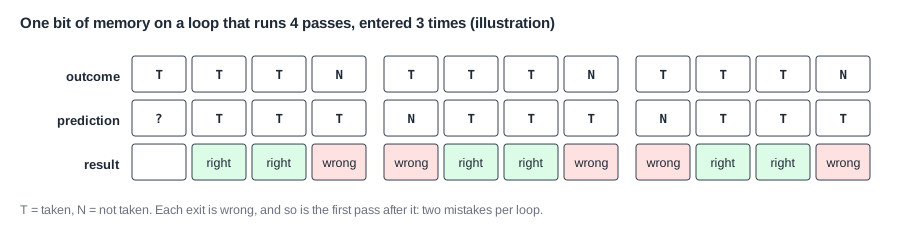
Every time the loop finishes, the prediction is wrong, which is unavoidable. But the bit then flips to "not taken", so the first branch of the next entry into the loop is also wrong. One surprise causes two mistakes. For a loop of 4 passes, half of those mistakes could have been avoided, and accuracy is 50 percent, worse than just predicting taken.
Two-Bit Counters
The fix is a little inertia, so that one surprise does not change the prediction. A two-bit saturating counter counts from 0 to 3. It goes up when the branch is taken and down when it is not, and it stops at either end instead of wrapping around, which is what "saturating" means. The top bit is the prediction:
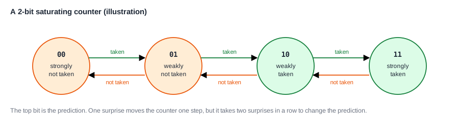
Now the loop exit moves the counter from strongly taken to weakly taken, and the prediction stays "taken", so the next entry into the loop is predicted correctly. Each loop costs one mistake instead of two. Why not use more bits? Studies since the early 1980s have shown that two bits gives nearly all of the gain, and going to three or more rarely helps.
On real programs, the improvement shows up where loops are short. In a model of a checksum whose inner loop runs a few passes per byte, one bit was right 80 percent of the time and two bits 90 percent. A bubble sort went from about 79 to about 84 percent.
The Bimodal Predictor
A bimodal predictor is a table of two-bit counters, indexed by the low bits of the branch's address. It needs no tags: at fetch, the low bits of the PC select one counter, and its top bit is the prediction. When the branch is resolved, the same counter is updated.
The name comes from the fact that most branches are bimodal: each is either nearly always taken or nearly always not taken. Counters settle quickly into a strong state and stay there. The table costs very little. A table of 1,024 counters is only 256 bytes.
Aliasing
Since there are no tags, two branches whose addresses share the same low bits use the same counter. This is aliasing, or interference. If they both go the same way, no harm is done. If one is nearly always taken and the other nearly always not taken, they fight over the counter, and both suffer. A larger table reduces this, but with sharply diminishing returns once there are enough counters for the active branches. In a model on small programs, 16 counters already gave the same result as 4,096 on five of six programs, because those programs have only a few branches. Predictor Accuracy and Sizing looks at this in detail.
Quick Check
Q: A two-bit counter starts at 11 (strongly taken). The branch outcomes are N, N, T, T, N. What is predicted each time, and how many are right?
Show Answer
Counter 11 predicts T, wrong, counter goes to 10. Predicts T, wrong, goes to 01. Predicts N, wrong (T), goes to 10. Predicts T, right, goes to 11. Predicts T, wrong (N), goes to 10. One right out of five: an unlucky sequence for a counter, which works best on branches that mostly go one way.
What One Counter Cannot See
A counter records a tendency: mostly taken or mostly not. It cannot predict a pattern. A branch that goes T, N, T, N in strict alternation is perfectly predictable to a person, but a two-bit counter gets about half of it wrong. And a branch inside a short loop that always exits after 8 passes follows an exact pattern too: seven taken, one not taken, repeating. A counter misses every exit.
There is also a pattern between branches. Consider this C code:
if (x == 0) a = 1;        // branch 1
if (y == 0) b = 1;        // branch 2
if (x == y) c = 1;        // branch 3
If branches 1 and 2 both found zero, then x equals y and branch 3's outcome is settled. The outcome of branch 3 is correlated with the two before it. In 1992, researchers showed that using this kind of information raises accuracy a great deal, because real programs are full of it: a test repeated in slightly different form, a check that follows from an earlier check.
Global History
To use correlation, a predictor needs a record of what recent branches did. A global history register (GHR) is a shift register. After every branch, it shifts left and takes in one bit: 1 for taken, 0 for not taken. So the GHR holds the outcomes of the last n branches in the program, in order, whichever branches they were.
Now the predictor can use different counters depending on the recent history. In the code above, branch 3 reached after "both zero" uses one counter, and the same branch reached after "both non-zero" uses another. Each counter learns its own case. The branch that alternates does the same: after history ...N it uses one counter, after ...T another, and both become certain.
gshare
There are several ways to combine the address and the history into a table index. The simplest effective way was proposed by Scott McFarling in 1993: XOR them together. The result is called gshare:
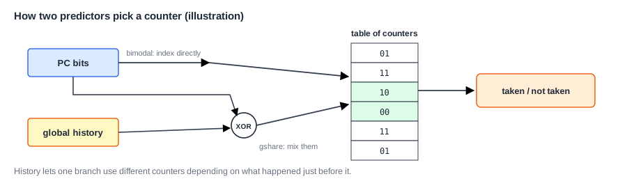
bimodal index = PC bits
gshare  index = PC bits XOR global history
Why XOR? Using only the history would mix up all the branches. Using the PC and history side by side would make a huge table that is mostly empty, because few combinations ever occur. XOR spreads the combinations that do occur across a table of a chosen size, sharing it well. It costs one small XOR gate per index bit.
The table still has no tags, so aliasing still happens, and now each branch uses several counters, one for each history it appears with. That takes longer to learn and needs a larger table. A gshare predictor is therefore often worse than bimodal when it is small, and better when it is large.
Results From Real Traces
A model of both predictors ran on six small programs, with 4,096 two-bit counters each:
| Program | Bimodal | gshare |
|---|---|---|
| array sum | 99.8% | 98.6% |
| memory copy | 99.8% | 98.7% |
| checksum | 90.0% | 99.7% |
| bubble sort | 84.4% | 86.1% |
| matrix multiplication | 70.9% | 72.5% |
| linked list | 86.5% | 85.7% |
The checksum shows the power of history. Its inner loop always runs the same number of passes, so the history tells the predictor exactly when the exit comes. That takes misses from 1 in 10 to about 1 in 300. On the simple array loops, gshare is slightly worse, because a very regular program spreads across many counters that each need a moment to warm up. And on the sort and the matrix program, neither does well, because the hard branches there depend on the data itself, and no history helps with random data. The numbers would differ on other programs; the pattern is typical.
Where Is This Used?
Small embedded cores often use a bimodal table of a few hundred entries, or a small gshare, because that gives most of the accuracy for a very small area. Mid-range cores use larger gshare-style predictors or combinations of predictors. The largest cores devote a large share of the front end to prediction, because at their pipeline depth a percent of accuracy can be worth several percent of performance.
Combining Predictors
Since bimodal is better on some branches and gshare on others, why not run both? A tournament predictor does that, with a third table of two-bit counters that learns, for each branch, which of the two has been doing better. The first well-known use was in a DEC Alpha processor of the late 1990s, which combined a global predictor with a local one that keeps a separate history for each branch.
Beyond gshare: TAGE and Perceptrons
Modern high-end predictors go further. TAGE (tagged geometric history length) keeps several tables, each using a longer history, from a few bits to hundreds. Its entries have partial tags, so aliasing is detected. The prediction comes from the table with the longest matching history. Short histories learn quickly, and long ones catch patterns that span many branches.
Perceptron predictors take a different approach, closer to a very small neural network. Each branch has a set of signed weights, one per history bit. The prediction is the sign of a sum, and the weights are trained on each outcome. This can use long histories without a table that grows exponentially, and versions of it have been used in real commercial processors.
The latest of these reach mispredictions of only a few per thousand instructions on many workloads. They use a surprising amount of storage: tens of kilobytes, against the 256 bytes of a simple bimodal table.
Quick Check
Q: A branch alternates T, N, T, N forever. How does a gshare predictor with two bits of history handle it, after it has warmed up?
Show Answer
The history before a T is always ...T,N, and the history before an N is always ...N,T (ignoring other branches). Those histories give two different indexes, so two different counters are used. One saturates at taken and the other at not taken, and the predictor is right every time.
How Predictors Are Updated
Prediction happens at fetch, but the outcome is known many cycles later, so updates are delayed. Several more predictions may be made in between. The global history cannot wait that long, or later branches would use stale history. So designs update the GHR speculatively at fetch with the predicted outcome, and save a copy at each branch. On a misprediction, they restore the copy and fix the last bit. Keeping history correct while on the wrong path is a detail that matters a lot to accuracy.
Common Mistakes
Mistake #1: Wrapping instead of saturating
A counter that wraps from 3 to 0 flips the prediction after one more taken branch, the exact opposite of what is wanted. Saturation is the whole point of the design.
Mistake #2: Sizing gshare's history wrongly
More history bits than the table can use spreads each branch thinly over too many counters. On small tables, a shorter history is often better. Test the history length along with the table size.
Mistake #3: Expecting history to help with random data
A branch that depends directly on random data has nothing to learn. If a program's accuracy will not rise, look at the code instead of the predictor, and consider removing the branch.
Practice Exercise
Challenge: Simulate by Hand
A loop runs 3 passes each time, so its branch goes T, T, N, repeating. Use a single two-bit counter starting at 10 (weakly taken). (a) Trace the prediction for 9 outcomes and count the mistakes. (b) What is the long-run accuracy? (c) Now give the predictor one history bit per outcome and enough history to see the last two outcomes, with one counter per pattern, all starting at 10. Which patterns occur, and what is the long-run accuracy after warming up?
Hint
For (c), the two previous outcomes before each branch can only be T,T or T,N or N,T.
Solution
(a) The counter goes 10, 11, 11 (predicts T, T, T; the third is wrong), then 10, 11, 11, and so on: it only drops to 10 on each N. The mistakes are the 3rd, 6th and 9th outcomes: 3 of 9. (b) 2 of 3, about 67 percent. (c) After T,T the outcome is always N. After T,N it is always T. After N,T it is always T. Each pattern has its own counter, which settles on the right answer, so accuracy reaches 100 percent. History turned a loop exit into a known event.
Summary
- A one-bit memory makes two mistakes per loop; a two-bit saturating counter makes one.
- A bimodal predictor is an untagged table of counters indexed by the PC, which suffers from aliasing.
- Global history records recent outcomes and lets a predictor use patterns and correlation between branches.
- gshare XORs history with the PC. On a checksum with a fixed inner loop it went from 90 to over 99 percent.
- Modern predictors such as TAGE combine many history lengths and use tens of kilobytes of storage.
