How RTL Simulation Works

Before you can debug a simulation failure, understand a race condition, or make sense of a waveform, you need to know what the simulator is actually doing under the hood. RTL simulators do not simply evaluate every gate at every nanosecond — they use an event-driven model that only recomputes logic when something changes. Understanding this model explains why delta cycles exist, why reading a signal immediately after writing it can give you a stale value, and why gate-level simulation is so much slower than RTL simulation. This article builds that foundation.

8 min read  |  Intermediate Level

What You'll Learn

• Why simulators use an event-driven model instead of evaluating every gate at every time step
• How the simulation event queue schedules and processes signal changes
• What delta cycles are and why combinational logic needs multiple zero-time iterations to settle
• Why event-driven simulation is efficient for typical RTL but slows down under dense activity

Why Not Evaluate Everything Every Nanosecond?

A naive approach to simulating a chip would be to evaluate every gate at every time step — pick a small time resolution, and at each tick, recompute the output of every logic cell in the design. This is called cycle-based or time-stepped simulation. For a design with millions of gates, it is hopelessly slow. Most gates do not change most of the time. Recomputing a stable AND gate 10 billion times to confirm its output is still 0 is pure waste.

Event-driven simulation solves this by only recomputing logic when something actually changes. A signal change — a clock edge, a data bus update, a reset assertion — creates an event. That event is placed in a queue, processed in timestamp order, and causes the simulator to recompute only the logic elements whose inputs were affected. Everything else is left alone. For typical RTL designs, this selective recomputation makes simulation orders of magnitude faster than full time-stepped evaluation.

A modern SoC simulation might contain tens of millions of logic gates, but during a typical bus transaction only a few hundred to a few thousand signals are toggling at any moment. Event-driven simulation exploits this sparsity — verification teams rely on it to run millions of clock cycles overnight in regression suites.

The Simulation Event Queue

At the heart of every RTL simulator is a data structure called the event queue (sometimes called the time wheel or event list). It stores a list of pending signal changes, each tagged with the simulation time at which that change should take effect. Simulation time first advances to the timestamp of the earliest pending event, that event fires and causes its signal to change, and the resulting downstream logic is then evaluated — potentially generating further events at the same or a later time.

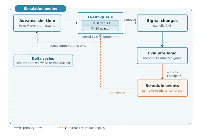
Processing an event means evaluating all logic that depends on the changed signal. If that evaluation produces a new output value on some downstream signal, another event is created and placed back in the queue, scheduled for the same or a later simulation time. This propagation continues until no more new events are generated at the current time. At that point, simulation time advances to the timestamp of the next event in the queue, and the cycle repeats.

The event queue sorts events by simulation time, not by circuit depth or fanout. The simulator does not traverse a netlist graph level by level — it processes whatever event is at the head of the queue, and that processing may generate further events at the same time or in the future.

Delta Cycles — Settling Combinational Logic

A question arises immediately: if a flip-flop output Q changes in response to a clock edge, and a combinational gate downstream depends on Q, does that gate's output update in the same simulation timestep? The answer is yes — but through a mechanism called delta cycles.

When an event causes a signal to change, any downstream events it generates are scheduled at the same simulation time but in the next delta cycle. A delta cycle is a zero-time iteration within a single simulation timestep. Simulation time does not advance during delta cycles — they are just additional passes within the same moment in simulated time, used to let combinational logic settle to a stable state.

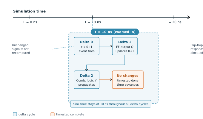
Consider what happens at a clock edge at T=10 ns. In delta cycle 0, the clock signal changes from 0 to 1. In delta cycle 1, the flip-flop processes the clock edge and its output Q updates. In delta cycle 2, the combinational logic fed by Q propagates and produces its new output. If that output feeds into further combinational logic, another delta cycle fires. This continues until no more changes occur — at which point the simulator considers the timestep complete and moves on.

Delta cycles are why you should never read a signal in the same timestep that you write it from a testbench. The write creates an event in delta 0, but the value you read immediately after (also in delta 0) has not yet propagated through the downstream logic. This is a common source of testbench race conditions, covered in detail in the next article on scheduling regions.

In theory, combinational feedback loops can cause delta cycles to keep firing indefinitely. Simulators protect against this with a delta cycle limit — if propagation has not settled after a configurable number of delta cycles (typically in the thousands), the simulator reports a zero-delay oscillation error. This almost always indicates a design bug: a combinational loop with no registered element to break the cycle.

Simulation Time vs Real Time

It is important to distinguish between simulation time and wall-clock time (the actual time your CPU spends running the simulation).

Simulation time is a counter maintained by the simulator. It is expressed in whatever time units the design specifies — nanoseconds, picoseconds, and so on. The simulator controls exactly when this counter advances: only when the event queue is empty at the current time and there are events pending at a later time. Simulation time has nothing to do with how long the simulation takes to run on the host machine.

Wall-clock time depends entirely on how much work the simulator has to do. If a testbench runs 1 million clock cycles with a 1 GHz clock, the simulated time span is 1 ms. That simulation might take 10 minutes of real CPU time or 2 hours, depending on the size of the design and the number of events per cycle. This ratio — simulated cycles per real second — is the simulation throughput, and it degrades as event density increases.

When Event-Driven Simulation Is Fast — and When It Is Not

Event-driven simulation is most efficient when activity is sparse: only a small fraction of signals change at each timestep. A CPU executing instructions, a memory controller processing periodic transactions, or a state machine sitting idle between bursts — these all have low average toggle rates, and event-driven simulation handles them well.

Performance degrades when activity is dense. Design patterns that stress the event-driven model include:

• Clock gating disabled across a large design — every register clocks every cycle, producing a flood of events at every rising edge.
• Wide random data buses — a 256-bit bus changing every cycle generates 256 separate signal-change events per timestep, each requiring downstream propagation.
• Gate-level simulation — simulating a synthesized netlist with millions of individual standard cells is far denser than RTL simulation, because each RTL assignment maps to many gate-level events.
• Power-aware simulation — switching power domains on and off creates cascades of isolation and level-shifter events throughout the design.

Gate-level simulation is typically 10–100x slower than RTL simulation for the same design, primarily because of the vastly higher event count. This is why sign-off gate-level simulations are run on a subset of test cases, not the full regression suite.

Verification teams at large chip companies track simulation throughput in millions of simulated cycles per hour across their compute farms. A 10% improvement in simulation performance can translate to days saved on a tapeout schedule. This is why emulation platforms — which run RTL on reconfigured FPGAs at MHz speeds — become essential for full-chip simulation of complex SoCs.

What the Simulator Actually Computes

When the simulator processes an event and evaluates a piece of logic, it is running compiled code on your host CPU — not some magical hardware engine. Modern simulators compile your SystemVerilog or Verilog source into optimized C++ or machine code as a preprocessing step. The resulting executable maintains the current value of every signal in memory, and each compiled logic block reads its input values, computes the result, and writes back to the output signal.

This compilation step is why simulation has a startup cost before the first event fires. It is also why changes to the RTL require a recompile (or an incremental recompile) before the next simulation run. The compiled code structure mirrors the RTL hierarchy — each module instance compiles to a distinct code region that can be called only when events arrive on its inputs.

Common Mistakes

// Flip-flop drives a combinational AND gate
always @(posedge clk)
    q <= d;        // sequential: q captures d on rising edge

assign y = q & en; // combinational: y follows q and en